SkillWisor

Introduction

Large Language Models (LLMs) have revolutionized natural language processing (NLP), enabling remarkable capabilities in text generation, translation, summarization, question answering, and various other language-related tasks. These models, exemplified by architectures like GPT (Generative Pre-trained Transformer), PaLM, LLaMA, Claude, and others, represent the culmination of decades of research in machine learning, computational linguistics, and artificial intelligence. They are characterized by their immense size (billions or even trillions of parameters) and their ability to learn complex patterns and relationships within vast amounts of text data during a self-supervised pre-training phase. This article provides a detailed exploration of LLM architecture, breaking down the fundamental concepts, design principles, key components, and implementation details, often illustrated with Python code examples using the PyTorch library.

The journey of language models has evolved significantly. Early approaches relied on statistical methods like n-grams, which predict the next word based on the previous n-1 words. While simple and effective for certain tasks, they struggled with capturing long-range dependencies and understanding context. The advent of neural networks led to Recurrent Neural Networks (RNNs) and their variants like Long Short-Term Memory (LSTM) and Gated Recurrent Units (GRUs). These models processed sequences step-by-step, maintaining a hidden state that theoretically captured past information. However, RNNs faced challenges with vanishing/exploding gradients, making it difficult to learn very long dependencies, and their sequential nature hindered parallelization during training.

A major breakthrough arrived with the introduction of the Transformer architecture by Vaswani et al. in their seminal 2017 paper, “Attention is All You Need.” This innovation replaced recurrence entirely with attention mechanisms, specifically self-attention. Self-attention allows the model to weigh the importance of different words in the input sequence when processing a specific word, regardless of their distance. This capability, combined with the architecture’s high parallelizability, enabled the training of much larger and deeper models on unprecedented amounts of data, leading directly to the era of LLMs.

As we delve into the architecture of these models, we’ll begin with the foundational steps of data preparation (tokenization) and representation (embeddings). We will then dissect the Transformer architecture, paying close attention to its core components: self-attention mechanisms, positional encoding, multi-head attention, feed-forward networks, layer normalization, and residual connections. We’ll explore why many modern LLMs adopt a decoder-only structure, discuss the pre-training objectives that imbue them with their general abilities, and touch upon scaling laws that govern their performance. Furthermore, we will cover advanced techniques optimizing performance and efficiency, training infrastructure considerations, common inference strategies, and methods for adapting pre-trained models to specific downstream tasks (fine-tuning). Finally, we’ll conceptually assemble these components into a mini-LLM structure and look towards the future of this rapidly evolving field.

Table of Contents

1. Foundation: Tokenization and Vocabulary
2. Word Embeddings and Token Representations
3. The Transformer Architecture
4. Self-Attention Mechanism: The Core of LLMs
5. Positional Encoding: Adding Sequential Information
6. Multi-Head Attention: Parallel Processing of Attention
7. Feed-Forward Networks in Transformers
8. Layer Normalization and Residual Connections
9. The Decoder-Only Architecture
10. Pre-training Objectives
11. Scaling Laws and Model Sizing
12. Advanced Techniques: Flash Attention, KV Caching, Rotary Embeddings
13. Training Infrastructure and Optimization
14. Inference Strategies
15. Fine-tuning Methodologies
16. Building a Mini-LLM from Scratch
17. Future Directions and Research Areas
18. Conclusion

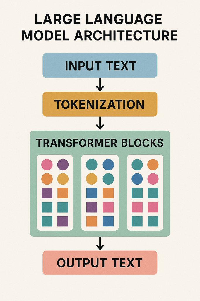
1. Foundation: Tokenization and Vocabulary

Before any text can be processed by a neural network, it must be converted into a numerical format that the model can understand. This process starts with tokenization, which involves breaking down the raw input text into smaller units called tokens. These tokens are then mapped to unique integer IDs based on a predefined vocabulary.

Challenges with Simple Tokenization

Early methods often tokenized text by splitting it into words based on spaces and punctuation. However, this approach has several drawbacks:

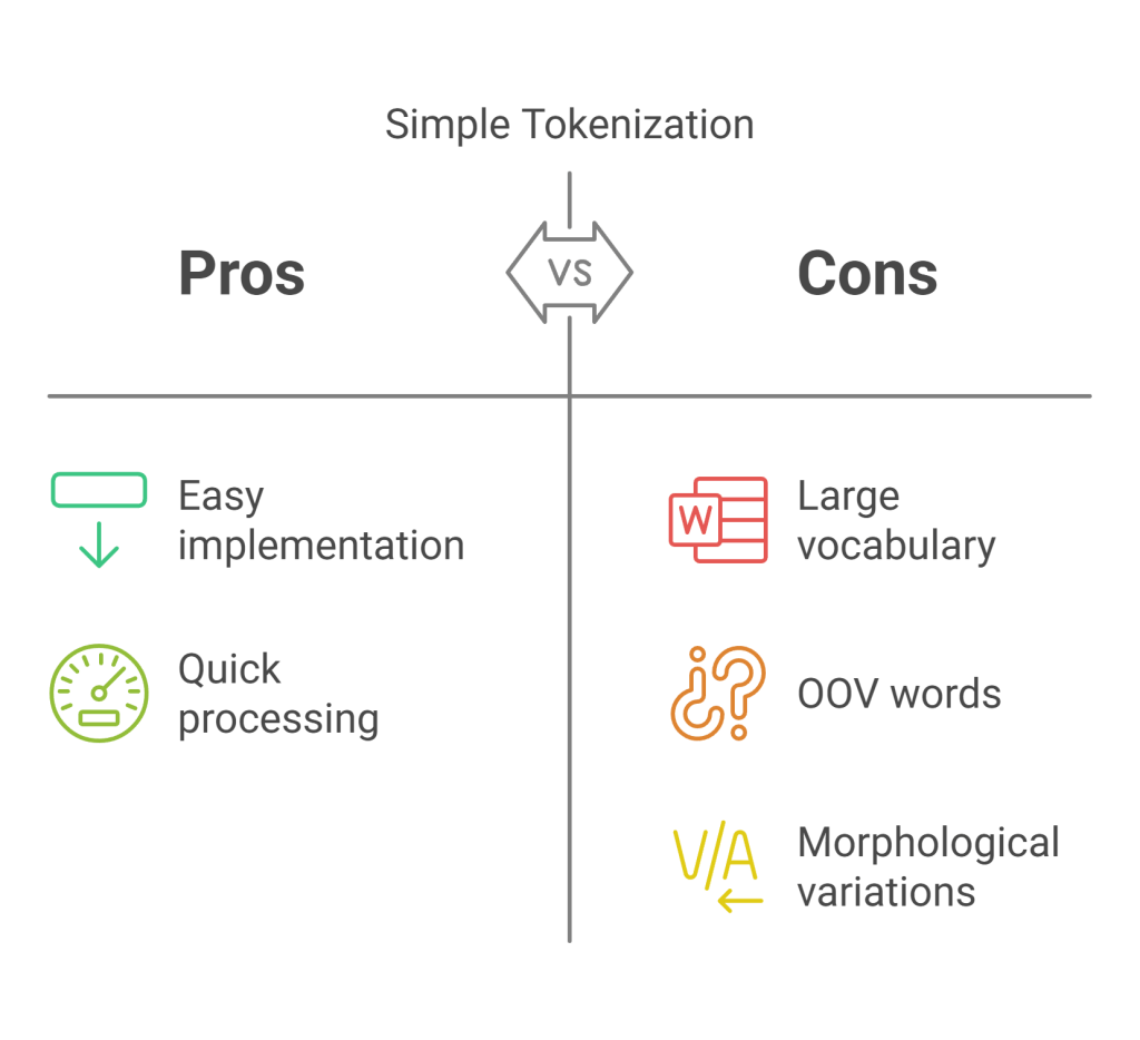
1. Large Vocabulary: Natural language contains hundreds of thousands of words, including variations (e.g., “run”, “running”, “ran”), proper nouns, and technical terms. A vocabulary covering every single word would become excessively large, leading to computational inefficiency and memory issues.
2. Out-of-Vocabulary (OOV) Words: No matter how large the vocabulary, there will always be words (new slang, typos, rare names) not present in it. These OOV words, often mapped to a special <UNK> (unknown) token, result in information loss.
3. Morphological Variations: Simple word splitting treats related words like “run” and “running” as entirely separate entities, failing to capture their shared root meaning efficiently.

Subword Tokenization

To address these challenges, modern LLMs almost universally employ subword tokenization algorithms. These methods break words down into smaller, semantically meaningful sub-units (like prefixes, suffixes, or common character sequences). The key idea is that common words remain as single tokens, while rare words are represented as sequences of subword tokens. This approach offers several advantages:

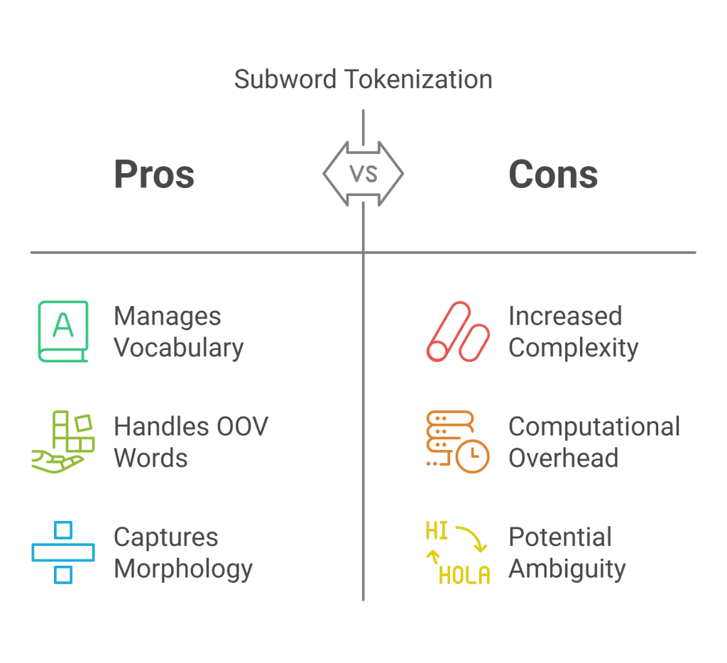
• Manages Vocabulary Size: It keeps the vocabulary size manageable (typically 30,000 to 100,000 tokens) while still being able to represent virtually any word or character sequence.
• Handles OOV Words: New or rare words can be constructed from known subword units, drastically reducing the occurrence of <UNK> tokens.
• Captures Morphology: Related words often share subword tokens (e.g., “running” might become “run” + “##ing”), potentially helping the model recognize semantic similarities.

Common subword tokenization algorithms include:

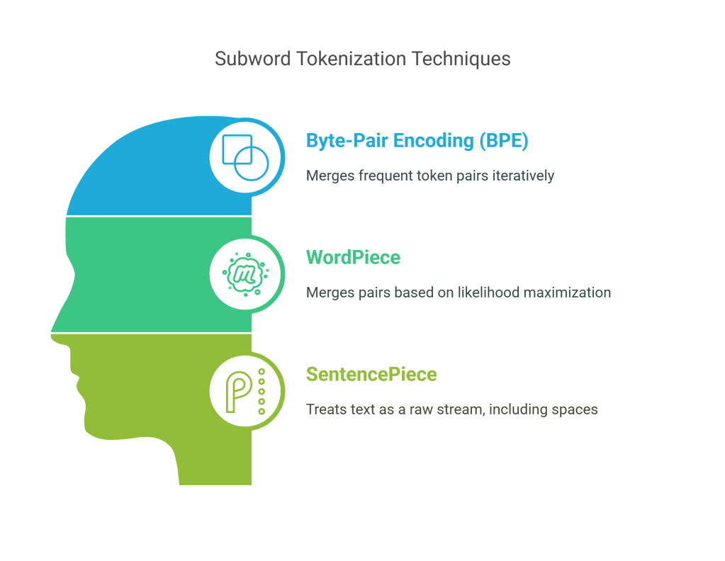
1. Byte-Pair Encoding (BPE):
   • Starts with a vocabulary of individual characters present in the training corpus.
   • Iteratively identifies the most frequent pair of adjacent tokens (initially characters) and merges them into a new, single token, adding it to the vocabulary.
   • This merging process repeats for a predefined number of steps or until the desired vocabulary size is reached.
   • Used in models like GPT-2, GPT-3.
2. WordPiece:
   • Similar to BPE but uses a likelihood-based criterion for merging pairs instead of raw frequency. It merges pairs that maximize the likelihood of the training data given the current vocabulary.
   • Starts with all characters and iteratively builds the vocabulary. Words are typically prefixed with “##” if they are continuations of a previous subword.
   • Used in models like BERT.
3. SentencePiece:
   • Treats the input text as a raw stream, including spaces. It tokenizes directly from raw text to a sequence of pieces, often encoding the space character itself (e.g., using U+2581).
   • Can operate directly on Unicode characters.
   • Provides both BPE and unigram language model tokenization modes. The unigram model starts with a large vocabulary and iteratively removes tokens that minimally impact the overall likelihood of the corpus representation.
   • Used in models like T5, LLaMA.

Vocabulary and Special Tokens

The result of the tokenization training process is a vocabulary: a mapping from each unique token (character, subword, or word) to an integer ID. LLM vocabularies also include special tokens for various control purposes:

• [PAD] or <pad>: Used for padding sequences in a batch to the same length.
• [CLS] or <s>: Sometimes used to represent the beginning of a sequence or for classification tasks (BERT).
• [SEP] or </s>: Used to separate distinct sequences (e.g., question and context in BERT) or mark the end of a sequence.
• [UNK] or <unk>: Represents tokens not found in the vocabulary (though minimized by subword tokenization).  
• [MASK]: Used in Masked Language Modeling objectives (BERT).
• [BOS] or <bos>: Beginning of sequence (often identical to <s>).
• [EOS] or <eos>: End of sequence (often identical to </s>).  

Example: BPE Tokenization (Conceptual Python)

Here’s a highly simplified conceptual implementation of the BPE learning process:

Python

import re, collections

def get_stats(vocab):
    """Counts frequency of adjacent pairs in words."""
    pairs = collections.defaultdict(int)
    for word, freq in vocab.items():
        symbols = word.split()
        for i in range(len(symbols)-1):
            pairs[symbols[i], symbols[i+1]] += freq
    return pairs

def merge_vocab(pair, v_in):
    """Merges the most frequent pair in the vocabulary."""
    v_out = {}
    bigram = re.escape(' '.join(pair))
    # Regex to find the pair, ensuring it's not part of a larger merged token already
    p = re.compile(r'(?<!\S)' + bigram + r'(?!\S)')
    for word in v_in:
        # Replace the pair with the merged token
        w_out = p.sub(''.join(pair), word)
        v_out[w_out] = v_in[word]
    return v_out

# --- Example Usage (Highly Simplified) ---
# 1. Initialize vocab with characters, space separated, plus end token </w>
corpus = {"low": 5, "lower": 2, "newest": 6, "widest": 3}
vocab = {'l o w </w>': 5, 'l o w e r </w>': 2, 'n e w e s t </w>': 6, 'w i d e s t </w>': 3}

num_merges = 10 # Desired number of merge operations

print("Initial vocab (char based):", vocab)

for i in range(num_merges):
    pairs = get_stats(vocab)
    if not pairs:
        break
    # Find the most frequent pair
    best = max(pairs, key=pairs.get)
    vocab = merge_vocab(best, vocab)
    print(f"Merge {i+1}: Merged {best} -> {''.join(best)}")
    print("Current vocab:", vocab)

# After training, the learned merges define the tokenizer rules.
# To tokenize "lowest":
# Start: l o w e s t </w>
# Merge 'e s': l o w es t </w>
# Merge 'es t': l o w est </w>
# Merge 'est </w>': l o w est</w>
# Merge 'l o': lo w est</w>
# Final tokens (assuming merges stopped here): ['lo', 'w', 'est</w>']

In practice, libraries like Hugging Face Transformers, tokenizers, or SentencePiece handle the complexities of training and applying these tokenizers efficiently.

Python

# Example using Hugging Face tokenizers library
from tokenizers import Tokenizer
from tokenizers.models import BPE
from tokenizers.trainers import BpeTrainer
from tokenizers.pre_tokenizers import Whitespace

# Initialize a tokenizer
tokenizer = Tokenizer(BPE(unk_token="[UNK]"))
tokenizer.pre_tokenizer = Whitespace() # Simple pre-tokenizer

# Trainer needs vocab_size and special_tokens
trainer = BpeTrainer(special_tokens=["[UNK]", "[CLS]", "[SEP]", "[PAD]", "[MASK]"], vocab_size=1000)

# Dummy files for training data
files = ["dummy_corpus.txt"]
with open("dummy_corpus.txt", "w") as f:
    f.write("This is the first sentence.\n")
    f.write("This is the second sentence with newer words.\n")
    f.write("Lowest and widest are comparative words.\n")

# Train the tokenizer
tokenizer.train(files, trainer)

# Save the tokenizer
# tokenizer.save("my_bpe_tokenizer.json")
# tokenizer = Tokenizer.from_file("my_bpe_tokenizer.json") # Load later

# Use the tokenizer
text = "This is the lowest sentence."
output = tokenizer.encode(text)

print(f"Text: {text}")
print(f"Token IDs: {output.ids}")
print(f"Tokens: {output.tokens}")

# Decode back
decoded_text = tokenizer.decode(output.ids)
print(f"Decoded Text: {decoded_text}")

2. Word Embeddings and Token Representations

Once text is tokenized into a sequence of integer IDs, these IDs must be converted into continuous vector representations that the neural network can process. This is the role of the embedding layer.

The Need for Embeddings

Integer IDs are categorical and arbitrary; the ID 500 has no inherent numerical relationship to ID 501. Neural networks, however, operate on real-valued vectors in geometric space. Embeddings provide a way to map discrete tokens into a continuous vector space where:

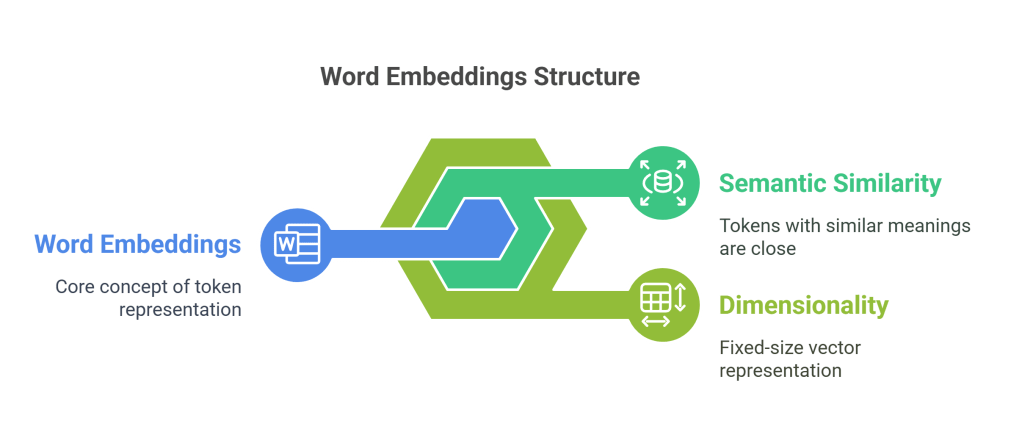
• Semantic Similarity: Tokens with similar meanings or that appear in similar contexts should have vectors that are close to each other in this space (e.g., the vectors for “king” and “queen” might be closer than “king” and “banana”).
• Dimensionality: Each token is represented by a dense vector of a fixed size (the embedding dimension, often denoted as d_model or d_embed), typically ranging from hundreds (e.g., 768 for BERT-base) to thousands (e.g., 12288 for GPT-3 175B). This is much more efficient than sparse representations like one-hot encoding, especially with large vocabularies.

Learned Embeddings

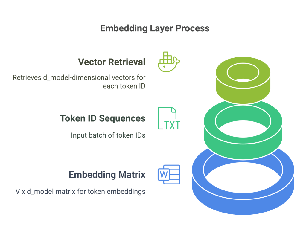
In modern LLMs, embeddings are learned during the model’s training process. The embedding layer is essentially a lookup table (a matrix) where each row corresponds to a token ID in the vocabulary, and the row itself is the embedding vector for that token.

• Embedding Matrix (W<sub>e</sub>): This matrix has dimensions Vtimesd_model, where V is the vocabulary size and d_model is the embedding dimension.
• Lookup Process: When the model receives a batch of token ID sequences (shape: [batch_size, sequence_length]), the embedding layer retrieves the corresponding d_model-dimensional vector for each token ID. The output is a tensor of shape [batch_size, sequence_length, d_{model}].

These embedding vectors are initialized randomly (or sometimes using pre-trained vectors like GloVe, though less common now for LLMs trained from scratch) and are then adjusted during training via backpropagation, just like any other parameter in the network. The model learns to place tokens in the embedding space such that the resulting vectors are useful for the downstream task (typically, predicting the next token).

Example: PyTorch Embedding Layer

Python

import torch
import torch.nn as nn

# --- Parameters ---
vocab_size = 50000  # Example vocabulary size
d_model = 768      # Embedding dimension (model dimension)
sequence_length = 128 # Length of input sequences
batch_size = 32     # Number of sequences processed in parallel

# --- Embedding Layer ---
embedding_layer = nn.Embedding(num_embeddings=vocab_size, embedding_dim=d_model)

# --- Example Input ---
# Batch of token ID sequences (random data for illustration)
# Shape: [batch_size, sequence_length]
input_ids = torch.randint(0, vocab_size, (batch_size, sequence_length))

# --- Embedding Lookup ---
# Output shape: [batch_size, sequence_length, d_model]
embeddings = embedding_layer(input_ids)

print(f"Shape of input token IDs: {input_ids.shape}")
print(f"Shape of output embeddings: {embeddings.shape}")
print(f"Embedding matrix shape (Weight): {embedding_layer.weight.shape}") # V x d_model

# --- How it works conceptually ---
# For the first token ID in the first sequence: input_ids[0, 0] = token_id
# The corresponding embedding vector is: embeddings[0, 0, :] = embedding_layer.weight[token_id]

This embedding tensor, containing rich vector representations for each token in the sequence, forms the initial input to the main body of the Transformer network. However, these embeddings only capture the identity of the tokens, not their position within the sequence, which is crucial for understanding meaning. This limitation is addressed by positional encoding.

3. The Transformer Architecture

The Transformer, introduced by Vaswani et al. (2017), forms the backbone of most modern LLMs. Its key innovation was relying entirely on attention mechanisms to draw global dependencies between input and output, dispensing with recurrence and convolutions. This design allows for significantly more parallelization during training and enables capturing long-range dependencies more effectively than RNNs.

Original Encoder-Decoder Structure

The original Transformer was designed for sequence-to-sequence tasks like machine translation and consisted of two main parts:

1. Encoder Stack: Processes the entire input sequence (e.g., the sentence in the source language). It comprises multiple identical layers, each containing two sub-layers:
   • Multi-Head Self-Attention: Allows each position in the encoder to attend to all positions in the input sequence.
   • Position-wise Fully Connected Feed-Forward Network: Applies the same transformation independently to each position.
2. Decoder Stack: Generates the output sequence one token at a time (e.g., the translated sentence). It also comprises multiple identical layers, each containing three sub-layers:
   • Masked Multi-Head Self-Attention: Allows each position in the decoder to attend to all positions up to and including itself in the output sequence (prevents looking ahead).
   • Multi-Head Cross-Attention: Allows each position in the decoder to attend to all positions in the encoder’s output (the representation of the input sequence).
   • Position-wise Fully Connected Feed-Forward Network.

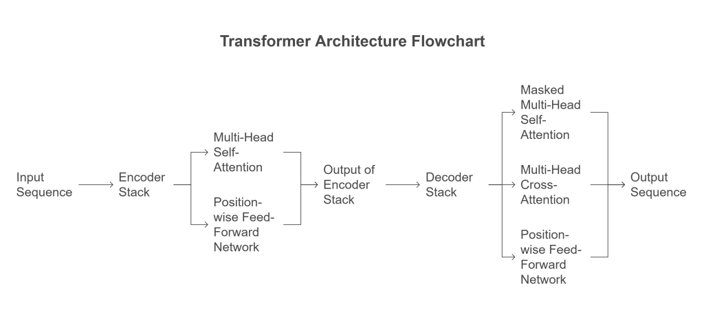
Residual connections and layer normalization are used around each sub-layer in both the encoder and decoder.

Variations: Encoder-Only, Decoder-Only

While the original architecture is powerful, different tasks benefit from variations:

1. Encoder-Only Models (e.g., BERT, RoBERTa): Use only the Transformer encoder stack. They are pre-trained (often using Masked Language Modeling) to build rich bidirectional representations of the input text. Excellent for natural language understanding (NLU) tasks like classification, named entity recognition (NER), and question answering where understanding the full context is key. The output is typically a representation for each input token or a pooled representation for the entire sequence.
2. Decoder-Only Models (e.g., GPT series, PaLM, LLaMA): Use only the Transformer decoder stack, usually without the cross-attention mechanism (as there’s no separate encoder output to attend to). They are pre-trained using a causal (next-token prediction) language modeling objective. This architecture is inherently generative and excels at text generation, open-ended dialogue, and few-shot learning. Most modern large-scale generative LLMs fall into this category.
3. Encoder-Decoder Models (e.g., T5, BART): Retain the full architecture, often pre-trained with objectives that involve reconstructing corrupted input (denoising autoencoders) or sequence-to-sequence tasks. They are versatile and perform well on both NLU and generation tasks, particularly conditional generation like translation and summarization.

This article will primarily focus on the components as they appear in the decoder-only architecture, which is prevalent in today’s generative LLMs. The core building block remains the Transformer layer (or block), which includes self-attention and feed-forward networks.

4. Self-Attention Mechanism: The Core of LLMs

The heart of the Transformer is the self-attention mechanism. It allows the model, when processing one token (or position) in the sequence, to dynamically weigh the importance of all other tokens in the same sequence and draw information from them. This contrasts sharply with RNNs, which process tokens sequentially and rely on hidden states to propagate information, often losing context over long distances.

Intuition: Asking Questions About the Sequence

Imagine you are processing the word “it” in the sentence: “The animal didn’t cross the street because it was too tired.” To understand what “it” refers to, you’d naturally look at other words in the sentence. Self-attention formalizes this intuition. For each token, the mechanism asks: “Which other tokens in this sequence are most relevant to understanding this token right here?”

Query, Key, Value Vectors

To implement this, self-attention uses three learned linear projections for each input token embedding (plus its positional information):

1. Query (Q): Represents the current token’s “question” or request for information. It asks: “What information do I need?”
2. Key (K): Represents the “label” or “identifier” of each token in the sequence. It responds to queries by saying: “This is the kind of information I hold.”
3. Value (V): Represents the actual content or meaning of each token. It provides the information if selected by the query-key interaction.

For an input sequence embedding tensor X of shape [sequence_length, d_model], three weight matrices W_Q, W_K, and W_V (each of shape d_modeltimesd_k, d_modeltimesd_k, and d_modeltimesd_v respectively, where often d_k=d_v=d_model/textnum_heads) are learned. The Q, K, V matrices for the entire sequence are computed as:

Q=XW_Q K=XW_K V=XW_V

Resulting shapes: Q is [sequence_length, d_k], K is [sequence_length, d_k], V is [sequence_length, d_v].

Scaled Dot-Product Attention

The core computation involves calculating an attention score between the Query of the current token and the Key of every other token (including itself). A common method is scaled dot-product attention:

1. Compute Dot Products: Calculate the dot product between the Query vector of the token being processed (Q_i) and the Key vector of every token (K_j) in the sequence. This measures the compatibility or relevance between the query and each key. Score_i,j=Q_icdotK_j. Performing this for all queries simultaneously gives a matrix of scores: Scores=QKT. (Shape: [sequence_length, sequence_length]).
2. Scale: Divide the scores by the square root of the dimension of the key vectors (sqrtd_k). This scaling prevents the dot products from growing too large (especially with high d_k), which could push the softmax function into regions with very small gradients, hindering learning. Scaled Scores = fracQKTsqrtd_k.
3. (Optional) Masking: For decoder self-attention (causal attention), apply a mask to the scaled scores before the softmax. This mask sets the scores corresponding to future positions (i.e., where ji) to negative infinity (-inf). This ensures that the attention calculation for a token i only depends on tokens 1 through i, preserving the auto-regressive property needed for generation.
4. Softmax: Apply the softmax function row-wise to the (masked) scaled scores. This converts the scores into probabilities (or weights) that sum to 1 for each query position i. These weights, denoted alpha_i,j, represent how much attention token i should pay to token j. AttentionWeights=softmax(fracQKTsqrtd_k+textMask). (Shape: [sequence_length, sequence_length]).
5. Weighted Sum of Values: Multiply the attention weights matrix by the Value matrix V. For each token i, this computes a weighted sum of all Value vectors in the sequence, where the weights are determined by the attention probabilities. The resulting vector is the output of the self-attention layer for token i, effectively aggregating information from the relevant parts of the sequence. Output=AttentionWeightscdotV. (Shape: [sequence_length, d_v]).

The formula is compactly written as: Attention(Q,K,V)=softmaxleft(fracQKTsqrtd_kright)V (Masking is applied inside the softmax for decoders).

Example: Conceptual Scaled Dot-Product Attention (Python/PyTorch)

Python

import torch
import torch.nn.functional as F
import math

def scaled_dot_product_attention(query, key, value, mask=None):
    """
    Computes scaled dot-product attention.

    Args:
        query: Query tensor (Batch, SeqLen_Q, Dim_K) or (Batch, Heads, SeqLen_Q, Dim_K/Heads)
        key: Key tensor (Batch, SeqLen_KV, Dim_K) or (Batch, Heads, SeqLen_KV, Dim_K/Heads)
        value: Value tensor (Batch, SeqLen_KV, Dim_V) or (Batch, Heads, SeqLen_KV, Dim_V/Heads)
        mask: Optional mask tensor (Batch, 1, SeqLen_Q, SeqLen_KV) or broadcastable.
              Mask values are typically 0.0 for positions to attend to and -inf for masked positions.

    Returns:
        output: Attention output tensor (Batch, SeqLen_Q, Dim_V) or (Batch, Heads, SeqLen_Q, Dim_V/Heads)
        attn_weights: Attention weights tensor (Batch, SeqLen_Q, SeqLen_KV) or (Batch, Heads, SeqLen_Q, SeqLen_KV)
    """
    d_k = query.size(-1) # Dimension of keys/queries

    # MatMul Q and K.T: (..., SeqLen_Q, Dim_K) x (..., SeqLen_KV, Dim_K) -> (..., SeqLen_Q, SeqLen_KV)
    scores = torch.matmul(query, key.transpose(-2, -1)) / math.sqrt(d_k)

    # Apply mask (if provided) before softmax
    if mask is not None:
        # Make sure mask has compatible shape or can be broadcasted
        # Typically adding -inf where mask is 0/False
         scores = scores.masked_fill(mask == 0, float('-inf')) # Often mask is 0 where we should mask

    # Apply softmax to get attention probabilities
    # Softmax is applied on the last dimension (SeqLen_KV)
    attn_weights = F.softmax(scores, dim=-1)

    # MatMul attention weights with V: (..., SeqLen_Q, SeqLen_KV) x (..., SeqLen_KV, Dim_V) -> (..., SeqLen_Q, Dim_V)
    output = torch.matmul(attn_weights, value)

    return output, attn_weights

# --- Example Usage (Simplified, single head) ---
batch_size = 1
seq_len = 5
d_k = 64 # Dimension of Key/Query vectors
d_v = 64 # Dimension of Value vectors (can be different, often same as d_k)

# Random Q, K, V for illustration
query = torch.randn(batch_size, seq_len, d_k)
key = torch.randn(batch_size, seq_len, d_k)
value = torch.randn(batch_size, seq_len, d_v)

# Example Causal Mask (for decoder self-attention)
# Prevents attending to future positions
# Shape: (seq_len, seq_len)
causal_mask_shape = (seq_len, seq_len)
# torch.triu: returns upper triangle of a 2D matrix. diagonal=1 means excluding diagonal
mask_tensor = torch.triu(torch.ones(causal_mask_shape), diagonal=1).bool()
# Unsqueeze for batch and head dimensions if needed for broadcasting
# Mask should be 0 for masked positions for masked_fill
# This creates a mask where future positions are True (masked)
# We need to invert it for the function above or adjust the function
# Let's adjust the function's expectation slightly for clarity here:
# Mask == True means position is MASKED
adjusted_mask = mask_tensor.unsqueeze(0).unsqueeze(1) # Shape: (1, 1, SeqLen, SeqLen)

# Call attention function (using a mask that's True for masked items)
def scaled_dot_product_attention_v2(query, key, value, mask=None):
    d_k = query.size(-1)
    scores = torch.matmul(query, key.transpose(-2, -1)) / math.sqrt(d_k)
    if mask is not None:
        scores = scores.masked_fill(mask, float('-inf')) # Fill where mask is True
    attn_weights = F.softmax(scores, dim=-1)
    output = torch.matmul(attn_weights, value)
    return output, attn_weights

output, attn_weights = scaled_dot_product_attention_v2(query, key, value, mask=adjusted_mask)

print("Input Query Shape:", query.shape)
print("Output Shape:", output.shape)
print("Attention Weights Shape:", attn_weights.shape)
# print("Attention Weights (first sequence):\n", attn_weights.squeeze())
# Note: attn_weights[b, i, j] is attention from query i to key j
# For causal mask, attn_weights[b, i, j] should be 0 if j > i
# Verify the mask worked (upper triangle should be zero after softmax)
print("Attention weights (upper triangle should be approx 0):\n", attn_weights.squeeze())

This self-attention mechanism is the fundamental operation allowing Transformers to model complex dependencies within sequences.

5. Positional Encoding: Adding Sequential Information

The self-attention mechanism, as described, is permutation-invariant. If you shuffle the input tokens, the attention scores between any two tokens remain the same (only their rows/columns in the attention matrix change). This means the model has no inherent sense of the order or position of tokens in the sequence, which is crucial for language understanding (e.g., “dog bites man” vs. “man bites dog”).

Positional Encoding (PE) is introduced to address this by injecting information about the absolute or relative position of each token into the input embeddings before they enter the main Transformer layers.  

Sinusoidal Positional Encoding (Original Transformer)

The original Transformer paper proposed using fixed sinusoidal functions of different frequencies for positional encoding. For a token at position pos and dimension i in the embedding vector (of size d_model), the PE value is calculated as:

PE_(pos,2i)=sinleft(fracpos100002i/d_modelright) PE_(pos,2i+1)=cosleft(fracpos100002i/d_modelright)

Where:

• pos is the position of the token in the sequence (0, 1, 2, …).
• i is the dimension index within the embedding vector ($0 \\le 2i \< d\_{model}$).
• d_model is the embedding dimension.

This generates a unique d_model-dimensional vector for each position. The key properties of this method are:

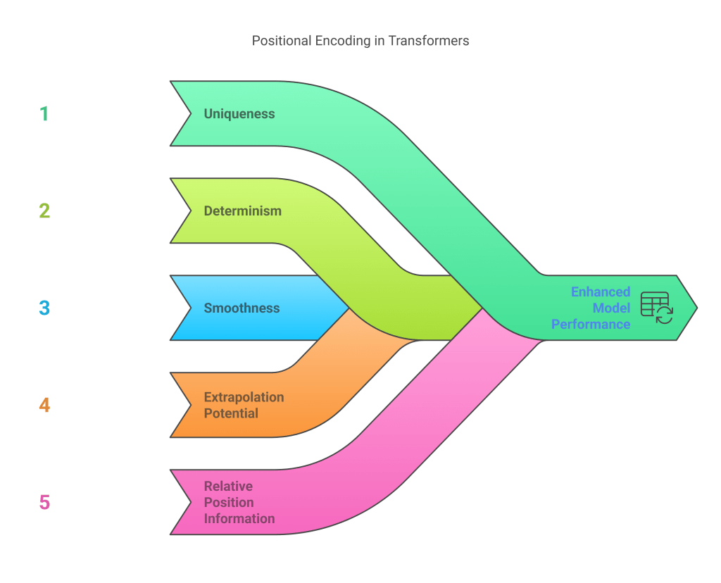
• Uniqueness: Each position gets a unique encoding.
• Determinism: The encodings are fixed and not learned.
• Smoothness: The values vary smoothly across positions.
• Extrapolation Potential: The sinusoidal nature might allow the model to generalize to sequence lengths longer than those seen during training (though performance often degrades).
• Relative Position Information: The formulation allows the model to easily learn relative positions, as PE_pos+k can be represented as a linear function of PE_pos.

These positional encoding vectors (shape: [max_sequence_length, d_model]) are typically added element-wise to the corresponding token embeddings (shape: [batch_size, sequence_length, d_model]).

X_final=TokenEmbeddings+PositionalEncodings

Learned Positional Embeddings

An alternative approach, used in models like BERT and GPT, is to use learned positional embeddings. Similar to token embeddings, a separate embedding matrix W_p of shape [max_sequence_length, d_model] is created. For each position index (0 to sequence_length - 1), the corresponding row vector from W_p is retrieved and added to the token embedding.

X_final=TokenEmbeddings+LearnedPositionalEmbeddings

These positional embeddings are initialized randomly and learned jointly with the rest of the model during training. This approach is simpler to implement and can potentially adapt better to the specific task and data, but it might not extrapolate as well to sequence lengths beyond the maximum seen during training.

Rotary Positional Embeddings (RoPE)

A more recent and increasingly popular method, especially in models like PaLM and LLaMA, is Rotary Positional Embedding (RoPE). Instead of adding positional information, RoPE modifies the Query and Key vectors within the attention mechanism itself, based on their absolute position.

Conceptually, RoPE applies a rotation matrix to the Query and Key vectors, where the angle of rotation depends on the token’s position m and the dimension index i. It operates on pairs of dimensions (2i,2i+1). If q_m is the query vector at position m, and k_n is the key vector at position n, RoPE effectively encodes their relative position (m−n) into the dot product q_mTR_Theta,m−nk<7>_n, where R is a rotation matrix dependent on the relative position. This inherently encodes relative positional information directly into the attention score calculation. RoPE has shown strong performance, particularly for long sequences.  

Example: PyTorch Sinusoidal Positional Encoding

Python

import torch
import torch.nn as nn
import math

class SinusoidalPositionalEncoding(nn.Module):
    def __init__(self, d_model: int, max_len: int = 5000):
        """
        Args:
            d_model: Dimension of the embeddings (must be even for simplicity here).
            max_len: Maximum sequence length supported.
        """
        super().__init__()
        self.d_model = d_model
        self.max_len = max_len

        # Create constant 'pe' matrix with values dependant on pos and i
        pe = torch.zeros(max_len, d_model)
        position = torch.arange(0, max_len, dtype=torch.float).unsqueeze(1) # [max_len, 1]
        # Calculate the division term: 10000^(2i/d_model)
        # Simplified: use exp(log(...)) for numerical stability
        div_term = torch.exp(torch.arange(0, d_model, 2).float() * (-math.log(10000.0) / d_model)) # [d_model/2]

        # Apply sin to even indices (0, 2, 4, ...)
        pe[:, 0::2] = torch.sin(position * div_term)
        # Apply cos to odd indices (1, 3, 5, ...)
        pe[:, 1::2] = torch.cos(position * div_term)

        # Add a batch dimension (1) so it can be broadcasted or easily added
        # Register as buffer so it's part of the model state but not trained
        self.register_buffer('pe', pe.unsqueeze(0)) # Shape: [1, max_len, d_model]

    def forward(self, x):
        """
        Args:
            x: Embeddings tensor (Batch, SeqLen, DimModel)

        Returns:
            Tensor with positional encoding added (Batch, SeqLen, DimModel)
        """
        # x.size(1) is the sequence length of the input batch
        # Add the positional encoding up to the sequence length of x
        # self.pe[:, :x.size(1), :] selects the PEs for the current sequence length
        x = x + self.pe[:, :x.size(1)]
        return x

# --- Example Usage ---
d_model = 512
max_seq_len_supported = 100
batch_size = 4
seq_len = 30 # Actual sequence length in this batch

# Token embeddings (dummy data)
token_embeddings = torch.randn(batch_size, seq_len, d_model)

# Create PE module
pos_encoder = SinusoidalPositionalEncoding(d_model, max_len=max_seq_len_supported)

# Add positional encoding
embeddings_with_pos = pos_encoder(token_embeddings)

print("Shape of token embeddings:", token_embeddings.shape)
print("Shape after adding positional encoding:", embeddings_with_pos.shape)

# --- Example: Learned Positional Embeddings ---
class LearnedPositionalEncoding(nn.Module):
    def __init__(self, d_model: int, max_len: int = 5000):
        super().__init__()
        self.pos_embedding = nn.Embedding(max_len, d_model)
        self.register_buffer('position_ids', torch.arange(max_len))

    def forward(self, x):
        """ x: (Batch, SeqLen, DimModel) """
        seq_len = x.size(1)
        # Get position IDs for the current sequence length: [SeqLen]
        position_ids = self.position_ids[:seq_len]
        # Look up embeddings for these IDs: [SeqLen, DimModel]
        # Add batch dimension for broadcasting: [1, SeqLen, DimModel]
        pos_enc = self.pos_embedding(position_ids).unsqueeze(0)
        x = x + pos_enc
        return x

# Usage similar to Sinusoidal PE

With positional information incorporated, the input embeddings are ready for the main Transformer layers.

6. Multi-Head Attention: Parallel Processing of Attention

While single scaled dot-product attention captures dependencies, the Multi-Head Attention (MHA) mechanism enhances this capability. Instead of performing a single attention function, MHA linearly projects the Queries, Keys, and Values h times (where h is the number of heads) with different, learned linear projections (weight matrices). It then performs the attention function in parallel for each of these projected versions (“heads”). Finally, the outputs of the individual heads are concatenated and linearly projected again to produce the final result.  

Rationale

The motivation behind MHA is to allow the model to jointly attend to information from different representation subspaces at different positions. A single attention head might average over different types of information, potentially diluting specific signals. With multiple heads, each head can potentially learn to focus on different aspects of the relationships between tokens:

• One head might focus on syntactic dependencies (e.g., subject-verb agreement).
• Another head might focus on semantic relationships (e.g., synonyms or related concepts).
• Another might focus on positional proximity.

By operating in parallel, these heads capture a richer set of dependencies.

Mechanism

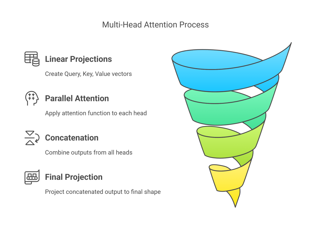
1. Linear Projections: For each head i (from 1 to h), create Query, Key, and Value vectors by projecting the input embeddings X (which include positional encodings) using learned weight matrices WQ_i, WK_i, WV_i. Q_i=XWQ_i K_i=XWK_i V_i=XWV_i Typically, the dimensions are set such that d_k=d_v=d_model/h. This keeps the total computation similar to a single head with full d_model dimensions.
2. Parallel Attention: Apply the scaled dot-product attention function independently to each head, producing h output vectors head_i: head_i=Attention(Q_i,K_i,V_i) (using the formula from Section 4, possibly with masking). Each head_i has shape [sequence_length, d_v].
3. Concatenation: Concatenate the outputs of all heads along the feature dimension: Concat=Concat(head_1,head_2,…,head_h) The resulting tensor has shape [sequence_length, h * d_v]. Since d_v=d_model/h, this shape is [sequence_length, d_model].
4. Final Linear Projection: Apply a final linear projection using another learned weight matrix WO (shape d_modeltimesd_model) to the concatenated output: MultiHeadOutput=ConcatcdotWO The final output has the desired shape [sequence_length, d_{model}], ready to be passed to the next layer.  

Example: PyTorch Multi-Head Attention Layer

Python

import torch
import torch.nn as nn
import torch.nn.functional as F
import math

# Assuming scaled_dot_product_attention function from Section 4 exists

class MultiHeadAttention(nn.Module):
    def __init__(self, d_model: int, num_heads: int):
        """
        Args:
            d_model: Total dimension of the model.
            num_heads: Number of attention heads. d_model must be divisible by num_heads.
        """
        super().__init__()
        assert d_model % num_heads == 0, "d_model must be divisible by num_heads"

        self.d_model = d_model
        self.num_heads = num_heads
        self.d_k = d_model // num_heads # Dimension of keys/queries per head
        self.d_v = d_model // num_heads # Dimension of values per head (can be same as d_k)

        # Linear layers for Q, K, V projections (can be combined into one large layer)
        self.W_q = nn.Linear(d_model, d_model) # Projects input to Qs for all heads
        self.W_k = nn.Linear(d_model, d_model) # Projects input to Ks for all heads
        self.W_v = nn.Linear(d_model, d_model) # Projects input to Vs for all heads

        # Final linear layer after concatenating heads
        self.W_o = nn.Linear(d_model, d_model)

    def split_heads(self, x, batch_size):
        """
        Splits the last dimension into (num_heads, d_k or d_v).
        Transposes the result to be (batch_size, num_heads, seq_len, d_k/d_v).
        Input shape: (batch_size, seq_len, d_model)
        Output shape: (batch_size, num_heads, seq_len, d_k/d_v)
        """
        x = x.view(batch_size, -1, self.num_heads, self.d_k) # Shape: (batch, seq_len, num_heads, d_k)
        return x.transpose(1, 2) # Shape: (batch, num_heads, seq_len, d_k)

    def forward(self, query_input, key_input, value_input, mask=None):
        """
        Args:
            query_input, key_input, value_input: Input tensors for Q, K, V.
                Shape: (batch_size, seq_len, d_model).
                In self-attention, these are typically the same tensor.
                In cross-attention (encoder-decoder), key/value come from encoder output.
            mask: Optional attention mask.

        Returns:
            output: Final multi-head attention output. Shape: (batch_size, seq_len, d_model)
            attn_weights: Attention weights from the scaled dot-product attention.
                          Shape: (batch_size, num_heads, seq_len, seq_len)
        """
        batch_size = query_input.size(0)

        # 1. Linear projections
        Q = self.W_q(query_input) # (batch, seq_len_q, d_model)
        K = self.W_k(key_input)   # (batch, seq_len_kv, d_model)
        V = self.W_v(value_input) # (batch, seq_len_kv, d_model)

        # 2. Split into multiple heads
        Q = self.split_heads(Q, batch_size) # (batch, num_heads, seq_len_q, d_k)
        K = self.split_heads(K, batch_size) # (batch, num_heads, seq_len_kv, d_k)
        V = self.split_heads(V, batch_size) # (batch, num_heads, seq_len_kv, d_v)

        # 3. Apply scaled dot-product attention for each head
        # scaled_attention_output shape: (batch, num_heads, seq_len_q, d_v)
        # attn_weights shape: (batch, num_heads, seq_len_q, seq_len_kv)
        scaled_attention_output, attn_weights = scaled_dot_product_attention(Q, K, V, mask)

        # 4. Concatenate heads
        # Transpose back: (batch, seq_len_q, num_heads, d_v)
        scaled_attention_output = scaled_attention_output.transpose(1, 2)
        # Concatenate: (batch, seq_len_q, d_model)
        concat_attention = scaled_attention_output.reshape(batch_size, -1, self.d_model)

        # 5. Final linear projection
        output = self.W_o(concat_attention) # (batch, seq_len_q, d_model)

        return output, attn_weights

# --- Example Usage ---
d_model = 512
num_heads = 8
batch_size = 4
seq_len = 60

mha_layer = MultiHeadAttention(d_model, num_heads)

# Dummy input (in self-attention, Q, K, V inputs are the same)
input_tensor = torch.randn(batch_size, seq_len, d_model)

# Create a causal mask for decoder self-attention
causal_mask = torch.triu(torch.ones(seq_len, seq_len), diagonal=1).bool()
# Expand mask to match attention weight shape (Batch, Heads, SeqLen_Q, SeqLen_KV)
# We need mask to be 0 where attention IS allowed, and -inf where it's NOT
# Or use masked_fill with boolean mask where True means MASKED
attention_mask = causal_mask.unsqueeze(0).unsqueeze(1) # (1, 1, SeqLen, SeqLen)
# Expand for batch size and heads (broadcasting usually handles this)
# attention_mask = attention_mask.expand(batch_size, num_heads, -1, -1)


# Pass input through MHA layer
# Using adjusted mask from previous example for clarity with masked_fill(mask is True)
output, attn_weights = mha_layer(input_tensor, input_tensor, input_tensor, mask=attention_mask)

print("Input tensor shape:", input_tensor.shape)
print("MHA Output shape:", output.shape)
print("Attention weights shape:", attn_weights.shape) # (Batch, Heads, SeqLen, SeqLen)

MHA is a critical component within each Transformer block, enabling the model to learn complex sequence representations.

7. Feed-Forward Networks in Transformers

Within each layer of the Transformer (in both encoder and decoder stacks), after the multi-head attention sub-layer, the output passes through a Position-wise Feed-Forward Network (FFN). This is a relatively simple component but plays a crucial role.

Structure and Function

The FFN consists of two linear transformations with a non-linear activation function in between. Importantly, this FFN is applied independently and identically to each position in the sequence. While the MHA layer allows tokens to interact and aggregate information, the FFN processes the representation at each position separately.

The typical structure is: FFN(x)=max(0,xW_1+b_1)W_2+b_2

Where:

• x is the output from the preceding layer (attention + residual connection + layer norm) for a specific position. Shape: [d_model].
• W_1, b_1 are the weights and bias of the first linear layer. W_1 has shape [d_model, d_ff].
• W_2, b_2 are the weights and bias of the second linear layer. W_2 has shape [d_ff, d_model].
• max(0,cdot) represents the ReLU activation function. Other activations like GELU (Gaussian Error Linear Unit) are also commonly used, especially in more recent models like GPT and BERT, often showing slightly better performance.

The intermediate dimension, d_ff (dimension of the feed-forward layer), is typically larger than d_model, often d_ff=4timesd_model. This expansion allows the model to project the information into a higher-dimensional space where it might be easier to separate or transform features, before projecting it back down to d_model.

Role in the Transformer

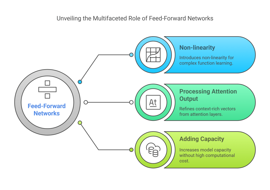
• Non-linearity: The activation function (ReLU, GELU) introduces non-linearity, which is essential for the model to learn complex functions beyond simple linear combinations.  
• Processing Attention Output: It processes the context-rich vectors produced by the MHA layer, potentially transforming and refining the aggregated information.
• Adding Capacity: The expansion to d_ff increases the model’s capacity to learn intricate patterns without drastically increasing computational cost compared to adding more attention layers.

Since the FFN operates position-wise, it can be implemented efficiently using 1×1 convolutions or standard dense layers applied across the sequence dimension.

Example: PyTorch Feed-Forward Network Module

Python

import torch
import torch.nn as nn
import torch.nn.functional as F

class PositionwiseFeedForward(nn.Module):
    def __init__(self, d_model: int, d_ff: int, activation=F.relu):
        """
        Args:
            d_model: Input and output dimension.
            d_ff: Inner dimension of the feed-forward layer.
            activation: Activation function (e.g., F.relu, F.gelu).
        """
        super().__init__()
        self.linear1 = nn.Linear(d_model, d_ff)
        self.linear2 = nn.Linear(d_ff, d_model)
        self.activation = activation
        # Dropout can also be added here for regularization
        # self.dropout = nn.Dropout(dropout_rate)

    def forward(self, x):
        """
        Args:
            x: Input tensor (Batch, SeqLen, DimModel)
        Returns:
            Output tensor (Batch, SeqLen, DimModel)
        """
        x = self.linear1(x)
        x = self.activation(x)
        # x = self.dropout(x) # Apply dropout if used
        x = self.linear2(x)
        return x

# --- Example Usage ---
d_model = 512
d_ff = 2048 # Typically 4 * d_model
batch_size = 4
seq_len = 60

ffn_layer = PositionwiseFeedForward(d_model, d_ff, activation=F.gelu) # Using GELU

# Dummy input (output from MHA + Add & Norm)
input_tensor = torch.randn(batch_size, seq_len, d_model)

# Pass through FFN
output_tensor = ffn_layer(input_tensor)

print("Input tensor shape:", input_tensor.shape)
print("FFN Output shape:", output_tensor.shape)

The combination of Multi-Head Attention and Position-wise Feed-Forward Networks forms the core computational units within each Transformer layer.

8. Layer Normalization and Residual Connections

Training very deep neural networks can be challenging due to issues like vanishing or exploding gradients and internal covariate shift (changes in the distribution of layer inputs during training). The Transformer architecture employs two crucial techniques to mitigate these problems and enable stable training of deep stacks of layers: Residual Connections and Layer Normalization.

Residual Connections (Skip Connections)

Introduced in ResNet models for computer vision, residual connections provide a shortcut path for the gradient and input data across a layer or block. In the Transformer, a residual connection is added around each of the two main sub-layers (Multi-Head Attention and Feed-Forward Network).

The output of a sub-layer is computed as: Output=Sublayer(Input)+Input

Where Input is the input to the sub-layer, and Sublayer is the function implemented by the sub-layer itself (e.g., MHA or FFN).

Benefits:

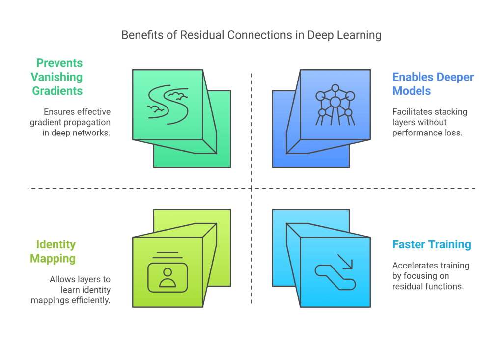
1. Gradient Flow: Allows gradients to flow more directly back through the network during backpropagation, preventing the vanishing gradient problem in deep networks. The network can easily learn an identity mapping if a layer is not beneficial, simply by driving the weights of the sub-layer towards zero.
2. Faster Training: Helps the network train faster by allowing layers to focus on learning the residual function (the difference needed) rather than the entire transformation from scratch.
3. Enables Deeper Models: Makes it feasible to stack many layers without performance degradation.

Layer Normalization

Normalization techniques aim to stabilize the distributions of activations within the network. While Batch Normalization (normalizing across the batch dimension) is common in CNNs, it can be less effective or trickier to apply in sequence models like Transformers, especially with variable sequence lengths and small batch sizes during inference.

The Transformer uses Layer Normalization (LayerNorm). LayerNorm normalizes the inputs across the features (the d_model dimension) for each individual data sample (sequence) in the batch independently.

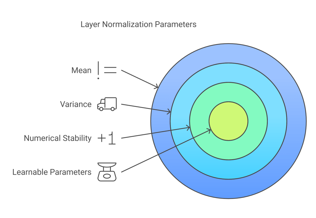
For an input vector x (representing a single token’s features at a specific position in a sequence), LayerNorm computes:

LN(x)=gammaodotfracx−musqrtsigma2+epsilon+beta

Where:

• mu is the mean of the elements in x.
• sigma2 is the variance of the elements in x.
• epsilon is a small constant added for numerical stability (e.g., 1e−5).
• gamma (gamma) and beta (beta) are learnable affine transformation parameters (scale and shift) of the same dimension as x. They allow the network to learn if normalization is actually beneficial or if it should scale/shift the normalized output.

Placement (Pre-LN vs. Post-LN):

In the original Transformer paper, Layer Normalization was applied after the residual connection: Output=LayerNorm(Sublayer(Input)+Input) (Post-LN)

However, subsequent research and popular implementations (like GPT-2/3, LLaMA) often use Pre-LN, where normalization is applied to the input of each sub-layer: Output=Input+Sublayer(LayerNorm(Input)) (Pre-LN)

Pre-LN has been found to often lead to more stable training, especially for very deep Transformers, as it ensures the inputs to the MHA and FFN sub-layers are consistently normalized, preventing activation magnitudes from exploding.

Putting it Together: A Transformer Block

A standard Transformer block (as found in many decoder-only LLMs using Pre-LN) typically follows this structure for an input X:

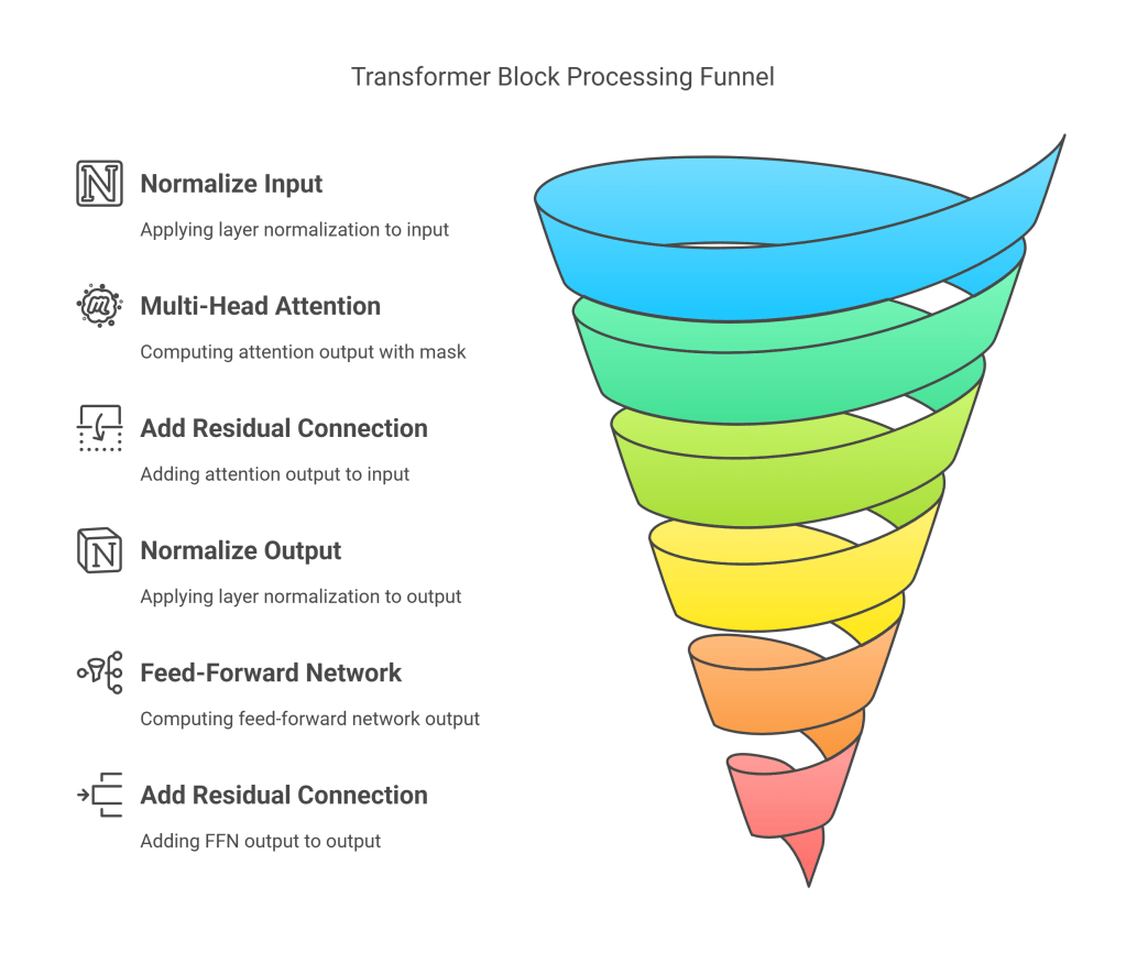
1. First Sub-layer (Multi-Head Self-Attention):
   • Normalize the input: X_norm1=LayerNorm(X)
   • Compute MHA: AttentionOutput=MultiHeadAttention(X_norm1,X_norm1,X_norm1,mask)
   • Add residual connection: X_res1=X+AttentionOutput
2. Second Sub-layer (Feed-Forward Network):
   • Normalize the output of the first sub-layer: X_norm2=LayerNorm(X_res1)
   • Compute FFN: FFNOutput=PositionwiseFeedForward(X_norm2)
   • Add residual connection: X_final=X_res1+FFNOutput

The output X_final is then passed as input to the next identical Transformer block. An LLM consists of stacking many (tens or even over a hundred) of these blocks.

Example: PyTorch Layer Normalization and Transformer Block (Pre-LN)

Python

import torch
import torch.nn as nn

# Assuming MultiHeadAttention and PositionwiseFeedForward classes exist

class TransformerBlock(nn.Module):
    def __init__(self, d_model: int, num_heads: int, d_ff: int, dropout_rate: float = 0.1):
        """
        Args:
            d_model: Model dimension.
            num_heads: Number of attention heads.
            d_ff: Inner dimension of FFN.
            dropout_rate: Dropout probability.
        """
        super().__init__()
        self.d_model = d_model
        self.num_heads = num_heads
        self.d_ff = d_ff

        # Layer Normalization layers
        self.norm1 = nn.LayerNorm(d_model)
        self.norm2 = nn.LayerNorm(d_model)

        # Multi-Head Attention layer
        self.mha = MultiHeadAttention(d_model, num_heads)

        # Position-wise Feed-Forward layer
        self.ffn = PositionwiseFeedForward(d_model, d_ff, activation=F.gelu) # Using GELU

        # Dropout layers (applied after MHA and FFN, before residual connection)
        self.dropout1 = nn.Dropout(dropout_rate)
        self.dropout2 = nn.Dropout(dropout_rate)

    def forward(self, x, mask=None):
        """
        Args:
            x: Input tensor (Batch, SeqLen, DimModel)
            mask: Optional attention mask for MHA.
        Returns:
            Output tensor (Batch, SeqLen, DimModel)
        """
        # --- First Sub-layer: Multi-Head Attention with Pre-LN ---
        # Residual connection stored
        residual1 = x
        # Apply LayerNorm before MHA
        x_norm1 = self.norm1(x)
        # Compute MHA (output and potentially attention weights)
        attn_output, _ = self.mha(x_norm1, x_norm1, x_norm1, mask=mask)
        # Apply dropout to MHA output
        attn_output = self.dropout1(attn_output)
        # Add residual connection
        x = residual1 + attn_output

        # --- Second Sub-layer: Feed-Forward Network with Pre-LN ---
        # Residual connection stored
        residual2 = x
        # Apply LayerNorm before FFN
        x_norm2 = self.norm2(x)
        # Compute FFN
        ffn_output = self.ffn(x_norm2)
        # Apply dropout to FFN output
        ffn_output = self.dropout2(ffn_output)
        # Add residual connection
        x = residual2 + ffn_output

        return x

# --- Example Usage ---
d_model = 512
num_heads = 8
d_ff = 2048
dropout = 0.1
batch_size = 4
seq_len = 60

transformer_block = TransformerBlock(d_model, num_heads, d_ff, dropout)

# Dummy input (output from previous layer or embedding layer)
input_tensor = torch.randn(batch_size, seq_len, d_model)

# Create a causal mask if this is a decoder block
causal_mask = torch.triu(torch.ones(seq_len, seq_len), diagonal=1).bool()
attention_mask = causal_mask.unsqueeze(0).unsqueeze(1) # (1, 1, SeqLen, SeqLen)

# Pass input through the Transformer block
output_tensor = transformer_block(input_tensor, mask=attention_mask)

print("Input tensor shape:", input_tensor.shape)
print("Transformer Block Output shape:", output_tensor.shape)

These techniques are fundamental to building and training the deep networks characteristic of modern LLMs.

9. The Decoder-Only Architecture

As mentioned earlier, while the original Transformer had both an encoder and a decoder, many of the most prominent large language models today, particularly those excelling at text generation (like GPT-3, PaLM, LLaMA, GPT-4), utilize a decoder-only architecture.

Structure

A decoder-only LLM essentially consists of:

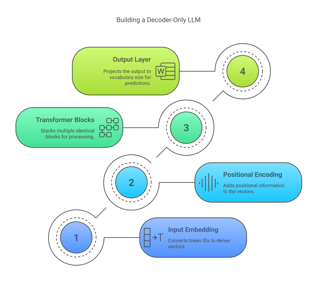
1. Input Embedding Layer: Converts token IDs to dense vectors (d_model).
2. Positional Encoding: Adds positional information (sinusoidal, learned, or rotary).
3. Stack of Transformer Decoder Blocks: Multiple identical blocks (as described in Section 8) are stacked sequentially. Each block contains:
   • Masked Multi-Head Self-Attention: Attends to previous positions in the sequence (including the current one). The masking ensures causality – the prediction for token t only depends on tokens 1 to t. Pre-LN is commonly used.
   • (No Cross-Attention): Unlike the original Transformer decoder, there’s no cross-attention layer because there is no separate encoder output to attend to.
   • Feed-Forward Network: Processes the output of the attention layer position-wise. Pre-LN is commonly used.
   • Residual connections around both sub-layers.
4. (Optional) Final Layer Normalization: Sometimes a final LayerNorm is applied after the last Transformer block.
5. Output Layer (Language Model Head): A final linear layer that projects the output representation (from the last Transformer block, dimension d_model) back to the vocabulary size (V). This produces logits (unnormalized log probabilities) for each token in the vocabulary at each position.
   • Shape transformation: [batch_size, sequence_length, d_model] -> [batch_size, sequence_length, vocab_size].

Why Decoder-Only for Generative LLMs?

1. Natural Fit for Autoregressive Generation: The core task of generative language modeling is predicting the next token given the preceding ones: P(w_t∣w_1,…,w_t−1). The masked self-attention mechanism in the decoder is perfectly suited for this, as it inherently prevents information flow from future tokens. The model learns to generate text token by token, conditioning on its own previous output.
2. Simplicity and Scalability: Compared to encoder-decoder models, the architecture is simpler, having only one type of block stack. This can simplify implementation and potentially make scaling (increasing depth/width) more straightforward.
3. Unified Pre-training and Fine-tuning: The same next-token prediction objective used for pre-training can often be directly applied or adapted for various downstream generative tasks (e.g., text completion, dialogue, summarization) with minimal architectural changes, often just through prompting or fine-tuning on specific datasets.
4. Effectiveness for Few-Shot/Zero-Shot Learning: Large decoder-only models pre-trained on vast text corpora have shown remarkable abilities to perform tasks described in natural language prompts without specific fine-tuning (zero-shot) or with only a few examples provided in the prompt (few-shot). The generative nature allows them to “complete” the task description given in the prompt.

How Prediction Works

During training, the model receives the input sequence and tries to predict the next token at each position. For an input sequence (w_1,w_2,…,w_T), the model computes output logits L (shape [batch_size, T, vocab_size]). The loss is typically calculated by comparing the predicted logits for position i (L_:,i,:) with the actual next token w_i+1 (using cross-entropy loss).

During inference (text generation):

1. Start with a prompt sequence (e.g., “Once upon a time”).
2. Feed the prompt through the model to get logits for the next token after the prompt.
3. Apply a sampling strategy (e.g., greedy decoding, nucleus sampling – see Section 14) to select the next token from the distribution defined by the logits.
4. Append the chosen token to the sequence.
5. Repeat steps 2-4, feeding the updated sequence back into the model until a desired length is reached or an end-of-sequence token is generated.

This autoregressive process, enabled by the masked self-attention in the decoder-only architecture, is fundamental to how these LLMs generate coherent and contextually relevant text.

10. Pre-training Objectives

The remarkable capabilities of LLMs stem largely from their pre-training phase. During pre-training, the model learns general language patterns, syntactic structures, semantic relationships, and world knowledge by processing massive amounts of unlabeled text data (often terabytes scraped from the internet, books, code, etc.). The specific pre-training objective defines the task the model performs on this unlabeled data to learn useful representations.

Causal Language Modeling (CLM) / Next-Token Prediction

This is the most common objective for decoder-only LLMs (GPT series, PaLM, LLaMA). The task is simple: predict the next token in a sequence given all the preceding tokens.

• Input: A sequence of tokens (w_1,w_2,…,w_t−1).
• Target: The next token w_t.
• Mechanism: The model processes the input sequence using masked self-attention (ensuring it only sees tokens up to position t−1 when predicting for position t). The output layer produces logits over the entire vocabulary for the t-th position.
• Loss: Typically Cross-Entropy Loss between the predicted probability distribution and the one-hot encoded vector representing the actual next token w_t. The total loss is usually the average loss over all positions in the sequence.

Loss=−sum_tlogP(w_t∣w_1,…,w_t−1)

By training on this objective over vast datasets, the model implicitly learns grammar, facts, reasoning patterns, and contextual understanding, as accurately predicting the next token often requires comprehending the preceding text.

Masked Language Modeling (MLM)

Primarily used for encoder-only models like BERT, MLM involves masking some percentage of the input tokens (e.g., 15%) and training the model to predict the original identity of these masked tokens based on the surrounding unmasked context.

• Input: A sequence with some tokens replaced by a special [MASK] token (e.g., “The [MASK] brown fox [MASK] over the lazy dog”).
• Target: The original tokens that were masked (e.g., “quick”, “jumps”).
• Mechanism: The model processes the entire corrupted sequence bidirectionally (using unmasked self-attention). The output representation corresponding to the [MASK] positions is fed into a linear layer to predict the original token.
• Loss: Cross-Entropy Loss calculated only over the masked positions.

MLM encourages the model to learn rich bidirectional context representations, making it very effective for NLU tasks. However, it’s less natural for direct text generation compared to CLM, and the artificial [MASK] token introduces a discrepancy between pre-training and downstream use (fine-tuning) where [MASK] typically doesn’t appear.

Variations and Other Objectives

• Permutation Language Modeling (PLM) (XLNet): Tries to combine benefits of CLM (autoregressive generation) and MLM (bidirectional context). It predicts tokens in a randomly permuted order instead of strictly left-to-right.
• Denoising Objectives (T5, BART): Used for encoder-decoder models. The input sequence is corrupted in various ways (masking spans of tokens, deleting tokens, shuffling sentences), and the model is trained to reconstruct the original, clean sequence. This trains both the encoder (to understand the corrupted input) and the decoder (to generate the clean output). T5 uses a unified text-to-text format where different tasks are cast as generating a target text string from an input text string.
• Contrastive Learning (ELECTRA): Uses a generator (small MLM model) to replace some input tokens and a discriminator (larger model) trained to distinguish which tokens were replaced by the generator versus the original tokens. This is often more sample-efficient than MLM.

For generative LLMs based on the decoder-only architecture, Causal Language Modeling remains the dominant pre-training objective due to its direct alignment with the autoregressive generation process. The sheer scale of data and model size allows CLM to learn surprisingly powerful and general representations.

11. Scaling Laws and Model Sizing

A key driver behind the recent success of LLMs has been the discovery and exploitation of scaling laws. These are empirical observations about the relationship between model performance (typically measured by the pre-training loss), model size (number of parameters, N), dataset size (D), and the amount of compute used for training (C).

The Basic Observation

Researchers found predictable power-law relationships: as you increase N, D, or C, the model’s test loss decreases smoothly and predictably, assuming the other factors are not bottlenecks.

$L(N, D, C) \\approx (\\frac{N}{N^*})^{-\\alpha\_N} + (\\frac{D}{D^*})^{-\\alpha\_D} + (\\frac{C}{C^\*})^{-\\alpha\_C} + L\_{\\infty}$

Where L is the loss, N, D, C are parameters, data, compute, and $N^*, D^*, C^\*$ are constants, alpha_N,alpha_D,alpha_C are scaling exponents, and L_infty is the irreducible loss.

This implies that simply making models bigger, feeding them more data, and training them for longer (using more compute) reliably leads to better performance, at least on the pre-training objective.

Kaplan et al. (OpenAI, 2020)

Early influential work showed that performance depends more strongly on model size (N) than dataset size or compute, provided the dataset is large enough and training is sufficient. They suggested scaling up model size (N) as the primary lever for improving performance, assuming compute budgets allow. They found roughly L(N)proptoN−0.076.

Hoffmann et al. (DeepMind, 2022) – “Chinchilla Scaling Laws”

This work refined the understanding by carefully studying the interplay between model size (N) and the number of training tokens (D). They found that for optimal performance given a fixed compute budget (C), both model size and dataset size should be scaled roughly in equal proportion.

• Previous large models (like GPT-3, Gopher) were likely undertrained relative to their size; they could have achieved the same performance with smaller models trained on much more data, or significantly better performance if trained for longer on more data.
• They proposed that for a given compute budget C, the optimal model size N_opt and number of tokens D_opt scale approximately as:
  • N_opt(C)proptoC0.5
  • D_opt(C)proptoC0.5
• This implies that for every doubling of model size, the training dataset size should also be doubled to maintain optimal compute allocation. Empirically, they suggested roughly 20 tokens per model parameter for optimal training (e.g., a 70B parameter model should be trained on ~1.4 Trillion tokens).

DeepMind trained Chinchilla (70B parameters) using this insight, training it on 1.4T tokens. Chinchilla significantly outperformed the much larger Gopher (280B parameters, trained on 300B tokens) and GPT-3 (175B, 300B tokens) on many downstream benchmarks, despite using the same compute budget as Gopher.

Implications

• Compute is Key: Training state-of-the-art LLMs requires enormous computational resources (thousands of GPUs/TPUs running for weeks or months).
• Data is Crucial: Access to massive, diverse, and high-quality datasets is essential. The Chinchilla laws highlight that scaling data alongside model size is critical for efficiency.
• Predictability: Scaling laws allow researchers to predict the performance gains from scaling up, helping justify the large investments required.
• Architectural Stability: The fact that scaling laws hold across different model sizes suggests the underlying Transformer architecture is robust and scalable.

These scaling laws have guided the development of subsequent LLMs, pushing towards training slightly smaller models (compared to the Kaplan et al. trajectory) but on significantly larger datasets (trillions of tokens).

12. Advanced Techniques and Optimizations

As LLMs grow larger, training and inference become increasingly computationally expensive and memory-intensive. Several advanced techniques have been developed to improve efficiency and performance:

1. FlashAttention / FlashAttention-2:
   • Problem: Standard self-attention requires materializing the large [SeqLen, SeqLen] attention matrix (QKT) in GPU High Bandwidth Memory (HBM), which is slow compared to on-chip SRAM. This makes attention memory-bound and inefficient, especially for long sequences.
   • Solution: FlashAttention reorganizes the attention computation to avoid writing the full attention matrix to HBM. It uses techniques like tiling (computing attention block by block) and recomputation (recomputing intermediate results instead of storing them) to keep intermediate results in the much faster SRAM.
   • Benefits: Significantly faster (up to ~9x speedup) and uses much less memory compared to standard attention, enabling training and inference on much longer sequences. FlashAttention-2 further optimizes parallelism and work partitioning for modern GPUs.
2. KV Caching (Key-Value Caching):
   • Problem: During autoregressive inference (generating token by token), standard self-attention recalculates Key (K) and Value (V) vectors for all previous tokens at each new step. This is highly redundant.
   • Solution: Cache the K and V vectors computed for previous tokens. At each step t, only compute the Q, K, V vectors for the new token t. Then, retrieve the cached K and V vectors for tokens 1..t−1 and concatenate them with the new K and V vectors before performing the attention calculation Attention(Q_t,[K_1..t−1,K_t],[V_1..t−1,V_t]).
   • Benefits: Dramatically speeds up inference generation time as the sequence grows, making latency much less dependent on the total generated length. The main cost becomes computing Q/K/V for the single new token and the final attention computation. Memory usage grows linearly with sequence length to store the cache.
3. Rotary Positional Embeddings (RoPE): (Mentioned in Section 5)
   • Mechanism: Instead of adding PE, RoPE applies position-dependent rotations to Query and Key vectors before the dot product in attention.
   • Benefits: Naturally encodes relative position information, integrates well with linear self-attention, and has shown strong empirical performance, especially in maintaining performance over long sequence lengths. Used in PaLM, LLaMA, and others.
4. Grouped-Query Attention (GQA) & Multi-Query Attention (MQA):
   • Problem: The KV cache (from technique 2) can become very large for models with many attention heads (h) and long sequences, as K and V vectors need to be stored for each head. Memory: 2 * num_layers * seq_len * d_model.
   • Solution (MQA): Share a single K and V projection across all heads within a layer. All heads use the same K and V vectors. Reduces KV cache size by a factor of h.
   • Solution (GQA): A compromise. Instead of 1 K/V head (MQA) or h K/V heads (MHA), use g K/V heads, where $1 \< g \< h$. Heads are grouped, and heads within a group share the same K/V projections. Reduces KV cache size by h/g.
   • Benefits: Significantly reduces the memory footprint of the KV cache during inference, allowing for longer contexts or larger batch sizes, often with minimal impact on model quality compared to MHA. GQA often provides a better quality/memory trade-off than MQA.
5. Mixture of Experts (MoE):
   • Problem: Scaling laws require huge models (trillions of parameters for SOTA), but dense models activate all parameters for every input token, making inference very slow and costly.
   • Solution: Replace some layers (typically the FFN) with MoE layers. An MoE layer consists of:
     • A Router (gating network): Determines which “expert(s)” should process the current token.
     • Multiple Experts: Independent FFNs (or other network types). Each expert has its own parameters.
   • Mechanism: For each token, the router selects a small number of experts (e.g., top-2). Only the parameters of the selected experts are activated and used for computation. The outputs of the selected experts are combined (often weighted by the router’s gating scores).
   • Benefits: Allows for models with a huge number of total parameters (trillions) while keeping the number of active parameters per token much smaller (similar to a dense model of manageable size). This leads to much faster training and inference compared to a dense model of the same total parameter count, while potentially achieving similar or better quality due to increased capacity. Examples: Switch Transformer, Mixtral 8x7B.
   • Challenges: Training stability, load balancing across experts, communication overhead in distributed settings.
6. Alternative Architectures (e.g., State Space Models – Mamba): While Transformer dominance persists, research explores alternatives. Mamba uses a structured state space model (SSM) backbone combined with a selection mechanism. It aims to achieve the sequence modeling power of Transformers but with linear scaling complexity in sequence length (compared to quadratic for standard attention) and potentially better handling of very long contexts.

These techniques, often used in combination, are crucial for pushing the boundaries of LLM scale and efficiency.

13. Training Infrastructure and Optimization

Training state-of-the-art LLMs is a massive engineering challenge requiring significant computational resources, sophisticated distributed training techniques, and careful optimization.

Hardware Requirements

• Accelerators: Training relies heavily on parallel processors optimized for matrix multiplication and floating-point operations.
  • GPUs (Graphics Processing Units): NVIDIA GPUs (A100, H100, B-series) are the most common hardware, offering high compute density and mature software ecosystems (CUDA, cuDNN).
  • TPUs (Tensor Processing Units): Google’s custom ASICs designed specifically for accelerating neural network training and inference. Often used for training Google’s own large models (PaLM, Gemini).
• Interconnect: High-bandwidth, low-latency interconnects (like NVIDIA’s NVLink and InfiniBand) are crucial for communication between accelerators in distributed training setups.
• Memory: Large amounts of GPU HBM are needed to hold model parameters, activations, gradients, and optimizer states. System RAM and fast storage (NVMe SSDs) are also important for data loading and checkpointing.

Distributed Training Techniques

A single accelerator cannot hold the parameters or process the data for large LLMs. Training must be distributed across hundreds or thousands of devices. Common parallelization strategies include:

1. Data Parallelism (DP):
   • Replicate the entire model on each device.
   • Each device processes a different mini-batch of data.
   • Gradients computed on each device are aggregated (e.g., averaged) across all devices using communication collectives (like AllReduce) before updating the model parameters (which are then synchronized back to all devices).
   • Simple to implement but memory usage per device is limited by the model size. Tools: PyTorch DistributedDataParallel (DDP), Horovod.
2. Tensor Parallelism (TP):
   • Split individual layers or tensors (parameters, activations) within the model across multiple devices.
   • For example, a large weight matrix in a linear layer or attention block can be partitioned column-wise or row-wise across devices.
   • Requires communication during the forward and backward pass of the layer (e.g., AllGather, ReduceScatter).
   • Allows fitting larger models than possible with DP alone, as model state is sharded. Often used within a node with fast interconnect (NVLink). Tools: Megatron-LM, DeepSpeed, NVIDIA NeMo.
3. Pipeline Parallelism (PP):
   • Partition the model layers sequentially across multiple devices. Device 1 computes layers 1-k, device 2 computes layers k+1 to m, etc.
   • Data flows through the devices in a pipeline fashion. Mini-batches are often split into micro-batches to keep the pipeline “bubbles” (idle time) low.
   • Reduces memory per device (each holds only a fraction of the layers) but can suffer from pipeline latency and requires careful load balancing. Tools: GPipe, PipeDream, DeepSpeed, NeMo.
4. ZeRO (Zero Redundancy Optimizer) (DeepSpeed):
   • A family of optimizations primarily focused on reducing memory redundancy in data parallelism.
   • Stage 1: Shards optimizer states across data-parallel devices (each device only holds/updates a partition of the optimizer state).
   • Stage 2: Additionally shards gradients across devices.
   • Stage 3: Additionally shards the model parameters themselves across devices (reconstructing layers on the fly as needed during forward/backward).
   • Allows scaling to much larger models under data parallelism by drastically reducing memory consumption per device.

Often, these techniques are combined (e.g., using TP within nodes, PP across nodes, and DP/ZeRO globally) to train the largest models efficiently.

Optimization Techniques

• Mixed Precision Training: Use lower-precision floating-point formats (like FP16 – half-precision or BF16 – bfloat16) for storing parameters, activations, and computing gradients, while often maintaining master weights and performing accumulation in FP32 (single-precision) for stability. Reduces memory footprint by ~2x and speeds up computation on hardware with specialized tensor cores. Requires loss scaling to prevent underflow of small gradient values in FP16.
• Optimizers: AdamW (Adam with decoupled weight decay) is a very common choice. Specialized optimizers like Sophia or Lion are sometimes explored. Managing optimizer states efficiently is crucial (handled by ZeRO or sharded optimizers).
• Learning Rate Scheduling: Carefully scheduling the learning rate during training is vital. Common schedules include a linear warmup phase (gradually increasing the LR from 0) followed by a decay phase (e.g., cosine decay, linear decay).
• Gradient Clipping: Limiting the maximum norm of gradients to prevent exploding gradients, especially early in training or with unstable data.
• Checkpointing: Regularly saving the model state (parameters, optimizer state, LR scheduler state) is essential for fault tolerance, as large training runs can take weeks or months and hardware failures can occur. Efficient asynchronous checkpointing to remote storage is needed.
• Activation Recomputation (Gradient Checkpointing): To save memory, instead of storing all activations needed for the backward pass, recompute them during the backward pass starting from strategically checkpointed activations. Trades compute for memory.

Training LLMs requires a confluence of expertise in ML algorithms, distributed systems, high-performance computing, and software engineering.

14. Inference Strategies

Once an LLM is pre-trained (and potentially fine-tuned), the next step is to use it for inference – typically, generating text based on a given prompt. Since the model outputs a probability distribution over the entire vocabulary at each step, various strategies exist for selecting the next token:

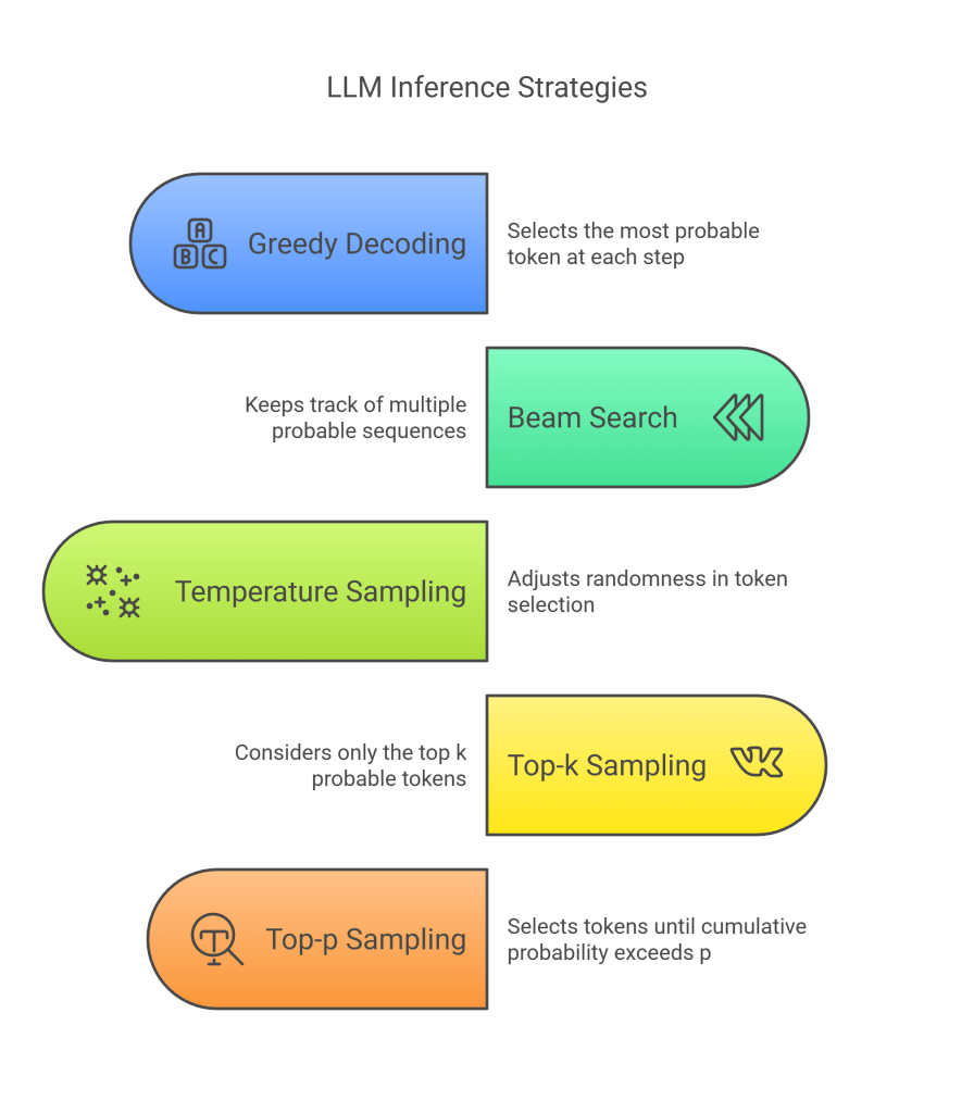
1. Greedy Decoding:
   • Mechanism: At each step, simply select the token with the highest probability (the argmax of the logits).
   • Pros: Simple, fast, deterministic.
   • Cons: Often leads to repetitive, dull, and unnatural-sounding text. Can get stuck in loops or suboptimal generation paths because it makes locally optimal choices without considering future consequences.
2. Beam Search:
   • Mechanism: Expands upon greedy search by keeping track of the k (beam width) most probable sequences (beams) at each step.
     • At step t, for each of the k current beams (sequences ending at t−1), generate probability distributions for the next token w_t.
     • Explore all ktimesV possible next tokens (where V is vocab size).
     • Calculate the cumulative probability (usually log probability sum) for all resulting sequences of length t.
     • Select the top k sequences based on their cumulative probability to become the new beams for step t+1.
   • Pros: Explores a larger search space than greedy decoding, often leading to higher probability (more “optimal” according to the model) and more coherent outputs, especially for tasks like translation or summarization where a single best output is desired.
   • Cons: Computationally more expensive (k times the work of greedy). Can still lead to repetitive text. Can favor common, safe phrases over more creative or interesting ones. Struggles with very long, open-ended generation.
3. Sampling Methods: Introduce randomness to select the next token, leading to more diverse and often more natural-sounding text, especially for creative tasks.
   • Temperature Sampling:
     • Mechanism: Rescale the logits before applying softmax: softmax(logits/T).
     • T is the temperature. T1 makes the distribution flatter (more uniform, more random sampling). $T \< 1$ makes it peakier (more like greedy). T=1 is standard softmax. Tto0 approaches greedy decoding.
     • After rescaling, sample from the resulting probability distribution.
     • Effect: Controls the randomness/creativity vs. predictability/focus of the output.
   • Top-k Sampling:
     • Mechanism: At each step, consider only the k most probable tokens. Truncate the distribution to these k tokens and redistribute their probabilities (normalize them to sum to 1). Then, sample from this reduced distribution (often combined with temperature).
     • Effect: Prevents sampling from very low-probability tokens in the long tail of the distribution, reducing the chance of nonsensical outputs, while still allowing for diversity among the top choices. k=1 is greedy decoding.
   • Top-p (Nucleus) Sampling:
     • Mechanism: Instead of a fixed number k, select the smallest set of tokens whose cumulative probability mass exceeds a threshold p (the nucleus). Sort tokens by probability, sum probabilities from highest downwards until the sum is gep. Truncate the distribution to this set and renormalize. Sample from this set (often combined with temperature).
     • Effect: Adapts the number of considered tokens based on the shape of the distribution. If the model is very confident (one token has high probability), the nucleus is small (similar to greedy). If the model is uncertain (probabilities spread out), the nucleus is larger, allowing more diversity. Often considered to produce higher quality and more diverse text than top-k.

Common Practice: For open-ended generation, combining Top-p (Nucleus) sampling with a moderate temperature (e.g., T=0.7, p=0.9) is a popular and effective strategy. Beam search might be preferred for tasks requiring more factual accuracy or coherence like translation. KV caching (Section 12) is almost always used during inference to speed up generation.

15. Fine-tuning Methodologies

While pre-training endows LLMs with general capabilities, fine-tuning adapts them to specific downstream tasks or desired behaviors (like following instructions or adopting a particular style).

1. Full Fine-tuning:
   • Mechanism: Initialize the model with pre-trained weights. Train the model further on a smaller, task-specific labeled dataset (e.g., question-answering pairs, summarization examples, instruction-following data). Update all model parameters using standard backpropagation.
   • Pros: Can achieve state-of-the-art performance on the target task by allowing the entire model to adapt.
   • Cons: Computationally expensive, requiring significant resources similar to pre-training (though on less data). Requires storing a full copy of the model weights for each task. Can suffer from “catastrophic forgetting,” where the model loses some of its general pre-trained abilities while specializing.
2. Parameter-Efficient Fine-tuning (PEFT): A family of techniques designed to adapt LLMs using far fewer trainable parameters, making fine-tuning much more efficient and manageable.
   • Adapter Tuning:
     • Mechanism: Freeze the pre-trained LLM weights. Insert small, new neural network modules (“adapters”) within each Transformer block (e.g., after the MHA and FFN sub-layers). Only train the parameters of these adapters on the task-specific data. Adapters typically have a bottleneck structure (project down, apply non-linearity, project up) with far fewer parameters than the main layers.
     • Pros: Drastically reduces the number of trainable parameters (e.g., &lt;1% of total). Faster training, much smaller storage overhead (only save adapters per task). Good performance, less prone to catastrophic forgetting.
     • Cons: Can slightly increase inference latency due to extra adapter layers. Performance might lag behind full fine-tuning on some tasks.
   • LoRA (Low-Rank Adaptation):
     • Mechanism: Freeze the pre-trained weights. For specific weight matrices in the LLM (often the Q, K, V, O projections in MHA), learn a low-rank update matrix. Instead of updating the original matrix W (shape dtimesk), learn two smaller matrices A (shape dtimesr) and B (shape rtimesk), where the rank rllmin(d,k). The update is W′=W+BA. Only A and B are trained.
     • Pros: Very parameter-efficient (similar to adapters). No inference latency increase, as the update BA can be merged with the original weight W after training. Strong empirical performance, often matching or exceeding adapters. Widely adopted.
     • Cons: Conceptual complexity slightly higher than adapters.
   • Prompt Tuning / Prefix Tuning:
     • Mechanism: Freeze the entire LLM. Learn a small set of continuous vector embeddings (“soft prompts” or “prefixes”) that are prepended to the input sequence embeddings. These learned vectors act as task-specific instructions or context for the frozen LLM. Only the prefix vectors are trained.
     • Pros: Extremely parameter-efficient (only train prefix vectors). Simple concept.
     • Cons: Can sometimes be less expressive or achieve lower performance than methods like LoRA or adapters, especially on complex tasks. Performance can be sensitive to hyperparameter choices (prefix length).
3. Instruction Tuning:
   • Mechanism: Fine-tune a pre-trained LLM on a large collection of “instructions” – examples of tasks described in natural language (e.g., “Translate this sentence to French: …”, “Summarize the following paragraph: …”, “Write a poem about …”). This dataset is often curated or generated synthetically. Typically uses full fine-tuning or PEFT methods.
   • Goal: Teach the model to follow instructions and generalize to new, unseen tasks described in a similar format. This is key to making base LLMs more usable as general-purpose assistants (like ChatGPT, Claude).
4. Reinforcement Learning from Human Feedback (RLHF):
   • Mechanism: A multi-stage process to align LLM behavior with human preferences, often used after instruction tuning.
     1. Collect Comparison Data: Generate multiple responses from the instruction-tuned model for various prompts. Have human labelers rank these responses from best to worst.
     2. Train a Reward Model (RM): Train a separate language model (often initialized from the instruction-tuned model) to predict the human preference score (reward) given a prompt and a response. The RM learns to approximate human judgment.
     3. Fine-tune LLM with RL: Use reinforcement learning (typically Proximal Policy Optimization – PPO) to fine-tune the instruction-tuned LLM. The LLM acts as the policy, generating responses. The RM provides the reward signal. The goal is to maximize the reward (human preference) while staying close to the original instruction-tuned model (using a KL divergence penalty) to avoid losing capabilities.
   • Pros: Explicitly optimizes for desired qualities like helpfulness, honesty, and harmlessness, as defined by human feedback. Can significantly improve the perceived quality and safety of LLM responses beyond supervised fine-tuning alone.
   • Cons: Complex and data-intensive process. Quality depends heavily on the quality and diversity of human feedback and the accuracy of the reward model. Can sometimes lead to “reward hacking” where the model optimizes the RM score in unintended ways. Alternatives like Direct Preference Optimization (DPO) are emerging.

PEFT methods, instruction tuning, and RLHF (or its alternatives) are crucial steps in transforming raw pre-trained LLMs into the helpful and capable AI assistants widely used today.

16. Future Directions and Research Areas

The field of Large Language Models is evolving at an incredible pace. Key areas of ongoing research and future directions include:

1. Scaling and Efficiency: While scaling laws hold, the cost is immense. Research focuses on:
   • More compute-efficient architectures (e.g., SSMs like Mamba, sparse MoEs).
   • Algorithmic improvements for attention (e.g., linear attention variants, further FlashAttention optimizations).
   • Hardware/software co-design for AI acceleration.
   • More data-efficient pre-training methods.
   • Quantization and distillation to create smaller, faster models for deployment.
2. Long Context Handling: Extending the effective context window beyond current limits (tens or hundreds of thousands of tokens) to handle entire books, codebases, or long conversations without losing information. This involves architectural changes (RoPE, ALiBi, attention variants) and efficiency improvements (FlashAttention, KV cache management).
3. Multimodality: Integrating information from multiple modalities beyond text, such as images, audio, and video (e.g., GPT-4V, Gemini). This involves learning joint representations and cross-modal attention mechanisms.
4. Reasoning and Planning: Improving the ability of LLMs to perform complex reasoning, mathematical problem solving, and multi-step planning. This might involve new architectures, incorporating external tools/knowledge bases, or improved training objectives that explicitly target reasoning skills.
5. Agentic AI: Developing LLMs that can act more autonomously, use tools (like calculators, search engines, APIs), plan sequences of actions, and interact with environments to achieve complex goals.
6. Alignment and Safety: Ensuring LLMs behave in ways that align with human values – being helpful, honest, and harmless. This includes research into:
   • More robust alignment techniques beyond RLHF (e.g., constitutional AI, debate, scalable oversight).
   • Understanding and mitigating biases present in training data.
   • Detecting and preventing harmful or untruthful outputs (hallucinations).
   • Ensuring controllability and interpretability.
7. Interpretability and Explainability: Understanding how LLMs make decisions and generate specific outputs. Developing methods to probe internal representations and attention patterns to gain insights into their reasoning processes.
8. Personalization and Adaptation: Efficiently adapting large pre-trained models to individual users, specific domains, or new tasks with minimal data and computation (advancing PEFT methods).
9. Evaluation: Developing better benchmarks and evaluation methodologies that accurately measure nuanced capabilities like reasoning, common sense, creativity, and safety, moving beyond simple task-specific metrics.

The field is dynamic, with breakthroughs occurring frequently, pushing the boundaries of what AI can achieve with language and related modalities.

Conclusion

Large Language Models, predominantly built upon the Transformer architecture, represent a significant milestone in artificial intelligence. Their ability to understand and generate human-like text stems from a combination of key architectural innovations and the power of scale.

We have journeyed through the core components: starting with tokenization to convert text into manageable units, followed by embedding layers that map these units into meaningful vector spaces. The introduction of positional encoding addresses the Transformer’s inherent lack of sequence awareness. The engine of the LLM is the stack of Transformer blocks, each employing multi-head self-attention to weigh the importance of different tokens and a position-wise feed-forward network to process information locally. Crucial elements like residual connections and layer normalization ensure stable training of these deep networks.

We explored the prevalence of the decoder-only architecture for generative tasks, driven by the causal language modeling pre-training objective. The remarkable performance of these models is strongly tied to scaling laws, demonstrating predictable improvements with increased model size, data, and compute. Advanced techniques like FlashAttention, KV caching, RoPE, GQA/MQA, and MoEs are vital for pushing efficiency and capability boundaries. Training these models requires massive infrastructure and sophisticated distributed training strategies, while inference relies on careful decoding methods like nucleus sampling. Finally, fine-tuning techniques, especially PEFT methods and alignment processes like instruction tuning and RLHF, adapt these powerful models for specific applications and user needs.

The architecture of LLMs is a testament to the progress in deep learning. While challenges remain in areas like reasoning, safety, efficiency, and true understanding, the ongoing research and rapid development cycles promise even more capable and impactful language models in the future. Understanding their underlying architecture is crucial for anyone looking to leverage, develop, or simply comprehend this transformative technology.