SkillWisor

Overview of the Data Science Life Cycle

Phase 1: Business Understanding

1.1 Defining Business Objectives

1.2 Assessing the Situation

1.3 Determining Data Science Goals

1.4 Project Planning

Phase 2: Data Acquisition

2.1 Identifying Data Sources

2.2 Data Collection Methods

2.3 Data Ingestion

2.4 Data Storage Considerations

Phase 3: Data Preparation

3.1 Data Cleaning

3.2 Data Integration

3.3 Data Transformation

3.4 Feature Engineering

3.5 Handling Imbalanced Data

Phase 4: Exploratory Data Analysis

4.1 Statistical Summaries

4.2 Data Visualization

4.3 Correlation Analysis

4.4 Hypothesis Generation

Phase 5: Data Modeling

5.1 Selecting Modeling Techniques

5.2 Building Models

5.3 Model Assessment

5.4 Hyperparameter Tuning

5.5 Ensemble Methods

Phase 6: Model Evaluation

6.1 Performance Metrics

6.2 Cross-Validation Techniques

6.3 Model Comparison

6.4 Addressing Overfitting and Underfitting

Phase 7: Model Deployment

7.1 Deployment Planning

7.2 Implementation Strategies

7.3 Integration with Existing Systems

7.4 Monitoring and Maintenance

Phase 8: Communication and Visualization

8.1 Storytelling with Data

8.2 Creating Effective Visualizations

8.3 Presenting to Different Audiences

8.4 Actionable Insights

Advanced Data Science Techniques

11.1 Vector Embeddings

11.2 One-Hot Encoding

11.3 SMOTE for Imbalanced Data

11.4 Feature Selection Methods

Ethics and Responsible Data Science

12.1 Privacy Considerations

12.2 Bias and Fairness

12.3 Transparency and Explainability

12.4 Ethical Guidelines

Case Studies

13.1 Predictive Maintenance in Manufacturing

13.2 Customer Churn Prediction

13.3 Healthcare Diagnosis Assistance

Industry-Specific Considerations

14.1 Healthcare

14.2 Finance and Banking

14.3 Retail and E-commerce

14.4 Manufacturing

Future Trends in Data Science

15.1 AutoML

15.2 MLOps

15.3 Edge AI

15.4 Federated Learning

Introduction

The data science life cycle represents the comprehensive journey from defining business problems to delivering actionable insights and solutions. This cyclical process combines domain expertise, programming skills, statistics, and machine learning to extract knowledge and value from data. Unlike a linear progression, the data science life cycle is iterative, with phases often revisited as new information emerges or business requirements evolve.

In today’s data-driven world, organizations across industries leverage data science to gain competitive advantages, optimize operations, enhance customer experiences, and drive innovation. Understanding the complete life cycle is essential for data scientists, analysts, business stakeholders, and technology leaders to effectively collaborate and maximize the value derived from data initiatives.

This comprehensive guide explores each phase of the data science life cycle in detail, from understanding business requirements to deploying and maintaining models in production. We’ll also examine specialized techniques like embeddings, one-hot encoding, and SMOTE, which play crucial roles in transforming raw data into meaningful insights. Additionally, we’ll discuss ethical considerations, industry-specific applications, and emerging trends shaping the future of data science.

Whether you’re a novice data scientist, an experienced practitioner, or a business leader overseeing data initiatives, this guide provides valuable insights into the methodologies, best practices, and challenges associated with the data science life cycle.

Overview of the Data Science Life Cycle

The data science life cycle encompasses a series of interconnected phases, each building upon the previous one while allowing for iteration and refinement. While various frameworks exist for conceptualizing this process—such as CRISP-DM (Cross-Industry Standard Process for Data Mining), TDSP (Team Data Science Process), and OSEMN (Obtain, Scrub, Explore, Model, iNterpret)—they all share fundamental elements.

At its core, the data science life cycle typically includes:

• Business Understanding: Defining objectives, assessing resources, and planning the project
• Data Acquisition: Identifying and collecting data from various sources
• Data Preparation: Cleaning, integrating, and transforming raw data
• Exploratory Data Analysis: Investigating patterns, relationships, and anomalies
• Data Modeling: Building predictive or descriptive models
• Model Evaluation: Assessing model performance and validity
• Model Deployment: Implementing models in production environments
• Communication and Visualization: Presenting findings and insights to stakeholders

What makes the data science life cycle distinct is its iterative nature. Insights gained during exploration might necessitate additional data collection; poor model performance might prompt revisiting feature engineering; and changing business requirements might require adjustments throughout the process. This flexibility enables continuous improvement and adaptation as projects evolve.

Let’s now delve into each phase in detail, examining the key activities, challenges, and best practices that define successful data science initiatives.

Phase 1: Business Understanding

The business understanding phase lays the foundation for the entire data science project. Without a clear understanding of business objectives and context, even the most sophisticated technical solutions may fail to deliver value. This initial phase bridges the gap between business stakeholders and data scientists, ensuring alignment on goals, expectations, and success criteria.

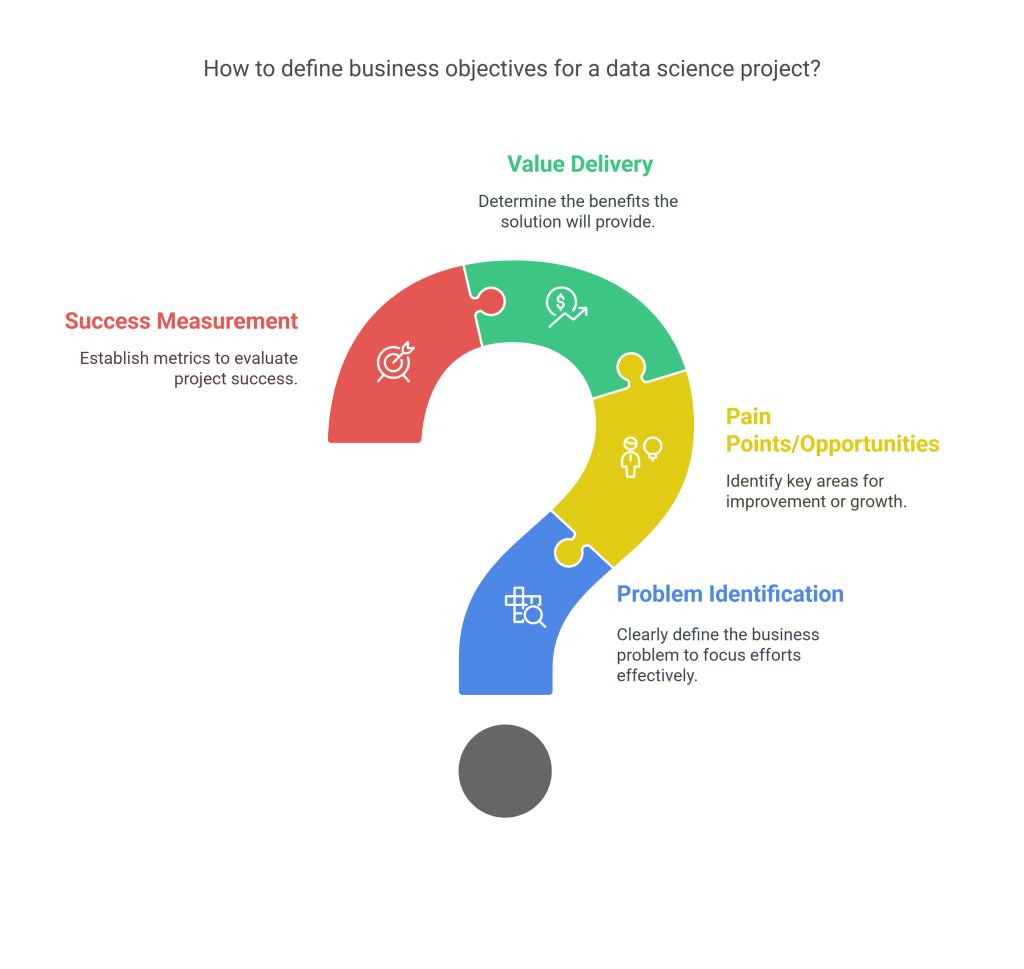
1.1 Defining Business Objectives

Every successful data science project begins with clearly articulated business objectives. These objectives should address the following questions:

• What business problem are we trying to solve?
• What are the key pain points or opportunities?
• What value will the solution deliver to the organization?
• How will success be measured from a business perspective?

Examples of well-defined business objectives include:

• Reducing customer churn by identifying at-risk customers and enabling proactive retention measures
• Optimizing inventory management to reduce costs while maintaining service levels
• Increasing conversion rates by personalizing customer experiences
• Detecting fraudulent transactions to minimize financial losses

Business objectives should be SMART (Specific, Measurable, Achievable, Relevant, and Time-bound). For instance, rather than simply stating “reduce customer churn,” a SMART objective would be “reduce monthly customer churn rate from 5% to 3% within six months by identifying high-risk customers and implementing targeted retention strategies.”

1.2 Assessing the Situation

Once business objectives are established, the next step involves assessing the current situation, including:

• Resource Inventory: Evaluate available data assets, technological infrastructure, human expertise, and time constraints. Understanding these resources helps set realistic expectations and identify potential bottlenecks.
• Constraints and Assumptions: Document business, legal, ethical, and technical constraints that might impact the project. For example, data privacy regulations like GDPR may limit data usage, or legacy systems might constrain implementation options.
• Risk Assessment: Identify potential risks and develop mitigation strategies. Risks might include data quality issues, stakeholder resistance, technical challenges, or changes in business priorities.
• Cost-Benefit Analysis: Estimate the costs associated with the project (personnel, technology, time) against the potential benefits to ensure the initiative delivers positive ROI.

1.3 Determining Data Science Goals

With business objectives and situational assessment in hand, data science goals can be formulated. These goals translate business objectives into technical terms, specifying what the data science project aims to accomplish:

• What type of analysis or models will be developed? (e.g., classification, regression, clustering, time series forecasting)
• What are the target variables or outcomes to predict or explain?
• What level of accuracy or performance is required for the solution to be valuable?
• What are the key questions the analysis should answer?

For example, if the business objective is to reduce customer churn, the data science goal might be “develop a classification model that predicts customers likely to cancel within the next 30 days with at least 80% precision and 70% recall.”

1.4 Project Planning

The final component of business understanding involves developing a comprehensive project plan that outlines:

• Project Roadmap: Define key milestones, deliverables, and timelines for each phase of the data science life cycle.
• Team Roles and Responsibilities: Clarify who will be responsible for various aspects of the project, from data collection to model deployment.
• Communication Plan: Establish how progress, findings, and challenges will be communicated to stakeholders throughout the project.
• Success Criteria: Define specific metrics and thresholds that will determine whether the project has achieved its objectives.
• Iteration Strategy: Plan for feedback loops and iterations to refine the approach based on intermediate findings.A well-executed business understanding phase creates alignment between technical teams and business stakeholders, establishes clear direction, and increases the likelihood of project success by ensuring that technical solutions address genuine business needs.

Phase 2: Data Acquisition

Data acquisition is the process of identifying, accessing, and collecting the data needed to address the business problem. This critical phase establishes the foundation for all subsequent analysis and modeling efforts. The quality, quantity, and relevance of the data gathered significantly impact the project’s success.

2.1 Identifying Data Sources

The first step in data acquisition involves identifying potential data sources that contain information relevant to the business problem. These sources typically fall into several categories:

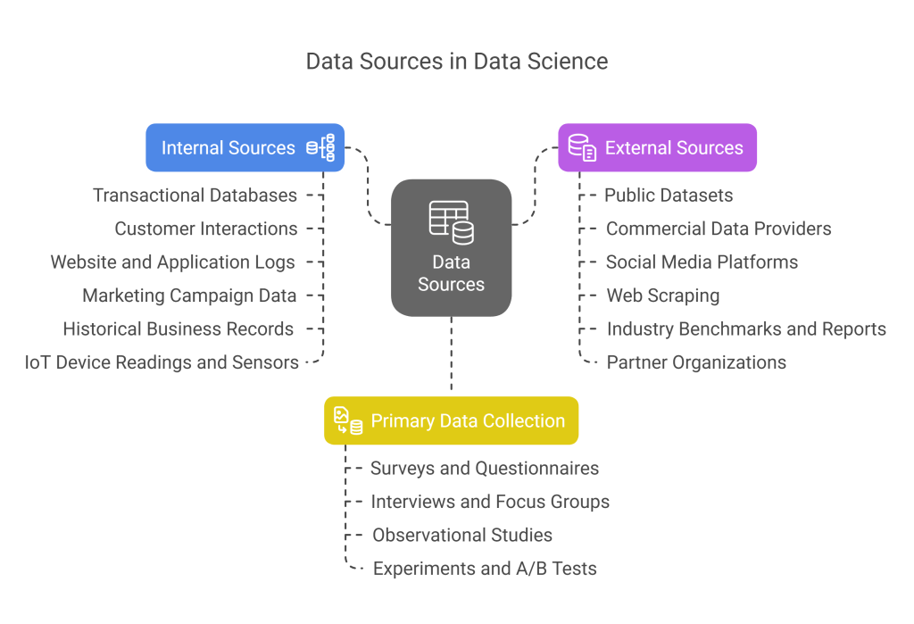
• Internal Sources:
  • Transactional databases (ERP, CRM, POS systems)
  • Customer interactions (call center logs, support tickets, chat transcripts)
  • Website and application logs
  • Marketing campaign data
  • Historical business records
  • IoT device readings and sensors
• External Sources:
  • Public datasets (government data, census information)
  • Commercial data providers
  • Social media platforms
  • Web scraping (with appropriate permissions)
  • Industry benchmarks and reports
  • Partner organizations
• Primary Data Collection:
  • Surveys and questionnaires
  • Interviews and focus groups
  • Observational studies
  • Experiments and A/B tests

When identifying data sources, consider factors such as data relevance, accessibility, quality, volume, freshness, and cost. It’s also important to assess whether the data contains the necessary information to answer your key questions and whether it covers the appropriate timeframe and population for your analysis.

2.2 Data Collection Methods

Once relevant data sources are identified, the next step is to implement appropriate collection methods:

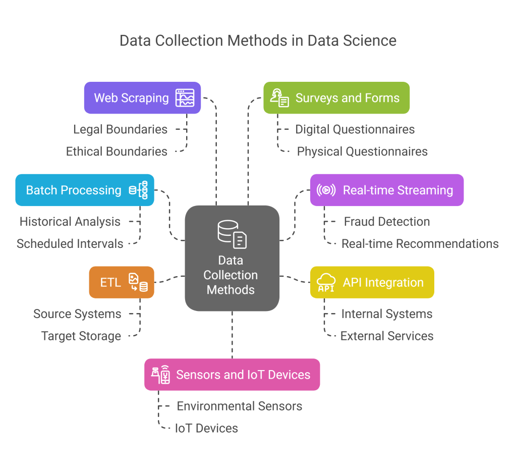
• Batch Processing: Extracting large volumes of data at scheduled intervals, often used for historical analysis or when real-time insights aren’t required.
• Real-time Streaming: Continuously collecting and processing data as it’s generated, essential for applications requiring immediate insights, such as fraud detection or real-time recommendations.
• API Integration: Accessing data through application programming interfaces provided by internal systems or external services.
• ETL (Extract, Transform, Load): Extracting data from source systems, applying initial transformations, and loading it into a target storage system.
• Web Scraping: Programmatically extracting data from websites, while respecting legal and ethical boundaries.
• Surveys and Forms: Collecting primary data directly from subjects through digital or physical questionnaires.
• Sensors and IoT Devices: Gathering data from physical devices and sensors deployed in the environment.

The collection method should align with data volume, velocity requirements, and technical constraints. For instance, high-velocity data from thousands of IoT sensors would require different collection methods than quarterly financial reports.

2.3 Data Ingestion

Data ingestion involves bringing data from various sources into a storage system where it can be processed and analyzed. Key considerations include:

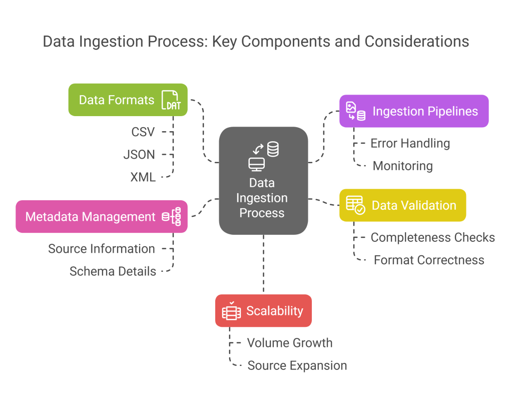
• Data Formats: Understanding and handling various data formats (CSV, JSON, XML, parquet, images, text, etc.) and ensuring compatibility with analysis tools.
• Ingestion Pipelines: Developing robust pipelines to automate the flow of data from sources to storage systems, including error handling and monitoring capabilities.
• Data Validation: Implementing checks during ingestion to verify data completeness, format correctness, and adherence to expected patterns.
• Metadata Management: Capturing metadata about the ingested data, including source, timestamp, schema information, and data lineage.
• Scalability: Ensuring ingestion processes can handle growing data volumes and additional data sources as the project evolves.

Modern data ingestion often leverages technologies like Apache Kafka for streaming data, Apache NiFi for dataflow management, or cloud-native services like AWS Glue, Google Cloud Dataflow, or Azure Data Factory.

2.4 Data Storage Considerations

The final aspect of data acquisition involves determining where and how to store the collected data:

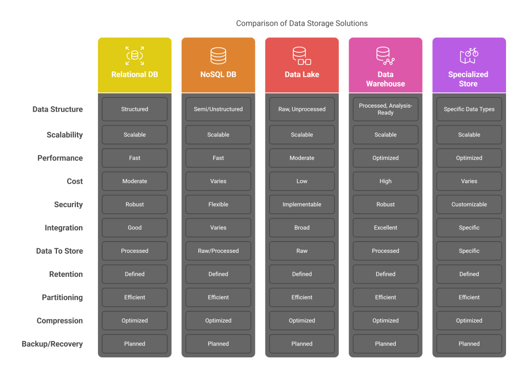
• Storage Types:
  • Relational databases (MySQL, PostgreSQL) for structured data with clear relationships
  • NoSQL databases (MongoDB, Cassandra) for semi-structured or unstructured data
  • Data lakes (using S3, Azure Blob Storage) for raw, unprocessed data
  • Data warehouses (Snowflake, Redshift, BigQuery) for processed, analysis-ready data
  • Specialized stores (time-series databases, graph databases) for specific data types
• Storage Architecture Considerations:
  • Scalability to accommodate growing data volumes
  • Performance requirements for data access and query speed
  • Cost considerations for storage and retrieval
  • Security and access control mechanisms
  • Compliance with data governance policies
  • Integration capabilities with analysis and modeling tools
• Storage Strategy:
  • Determine what data to store (raw vs. processed)
  • Establish data retention policies
  • Define partitioning strategies for efficient access
  • Implement compression to optimize storage utilization
  • Plan for backup and disaster recovery

Effective data acquisition establishes a solid foundation for analysis by ensuring that relevant, high-quality data is available in accessible formats. It requires close collaboration between data engineers, IT teams, and data scientists to balance technical constraints with analytical requirements.

Phase 3: Data Preparation

Data preparation, often consuming 60-80% of a data scientist’s time, transforms raw data into a format suitable for analysis and modeling. This critical phase addresses data quality issues, creates meaningful features, and ensures the dataset represents the problem domain accurately.

3.1 Data Cleaning

Data cleaning focuses on identifying and resolving quality issues that could undermine analysis:

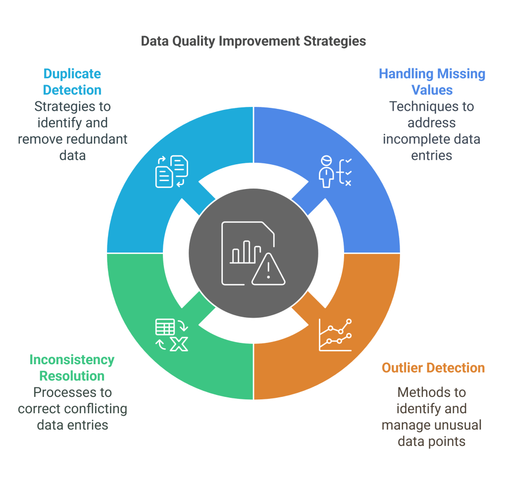
• Handling Missing Values:
  • Deletion: Removing records or features with missing values when data is sparse
  • Imputation: Filling missing values using mean, median, mode, or more sophisticated methods like k-NN or regression
  • Special values: Replacing missing values with a special indicator when missingness itself is informative
  • Multiple imputation: Generating several complete datasets with different imputed values to account for uncertainty
• Outlier Detection and Treatment:
  • Statistical methods: Using z-scores, IQR, or modified z-scores to identify values far from central tendencies
  • Visualization techniques: Box plots, scatter plots, and distribution plots to visually identify anomalies
  • Domain-based rules: Applying business logic to identify implausible values
  • Treatment options: Capping, transformation, removal, or special modeling approaches
• Inconsistency Resolution:
  • Standardizing formats (dates, addresses, phone numbers)
  • Resolving conflicting information across different data sources
  • Correcting logical inconsistencies (e.g., birth date after hire date)
  • Standardizing units of measurement
• Duplicate Detection and Removal:
  • Exact matching for identifying identical records
  • Fuzzy matching for identifying near-duplicates with slight variations
  • Record linkage techniques for identifying entities across different datasets

Data cleaning should be documented thoroughly, recording all decisions and their rationales. This documentation helps ensure reproducibility and provides context for other team members.

3.2 Data Integration

Data integration combines information from multiple sources into a unified view:

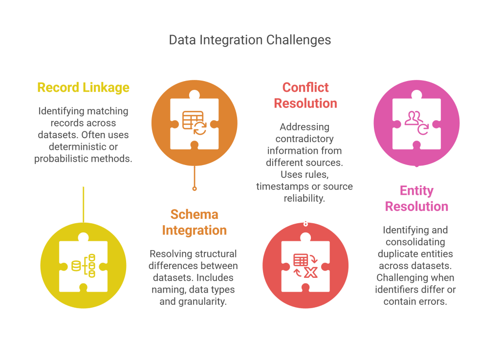
• Record Linkage: Identifying and matching records representing the same entity across different datasets, often using deterministic rules or probabilistic methods.
• Schema Integration: Resolving structural differences between datasets, including:
  • Naming conventions (e.g., “customer_id” vs. “cust_id”)
  • Data types (e.g., dates stored as strings vs. date objects)
  • Granularity differences (daily vs. monthly data)
• Conflict Resolution: Addressing contradictory information from different sources through rules, timestamps, source reliability ratings, or aggregation.
• Entity Resolution: Identifying and consolidating duplicate entities across datasets, particularly challenging when identifiers differ or contain errors.

Effective data integration creates a comprehensive view of the domain, enabling analyses that would be impossible with siloed data sources.

3.3 Data Transformation

Data transformation converts clean, integrated data into formats more suitable for analysis and modeling:

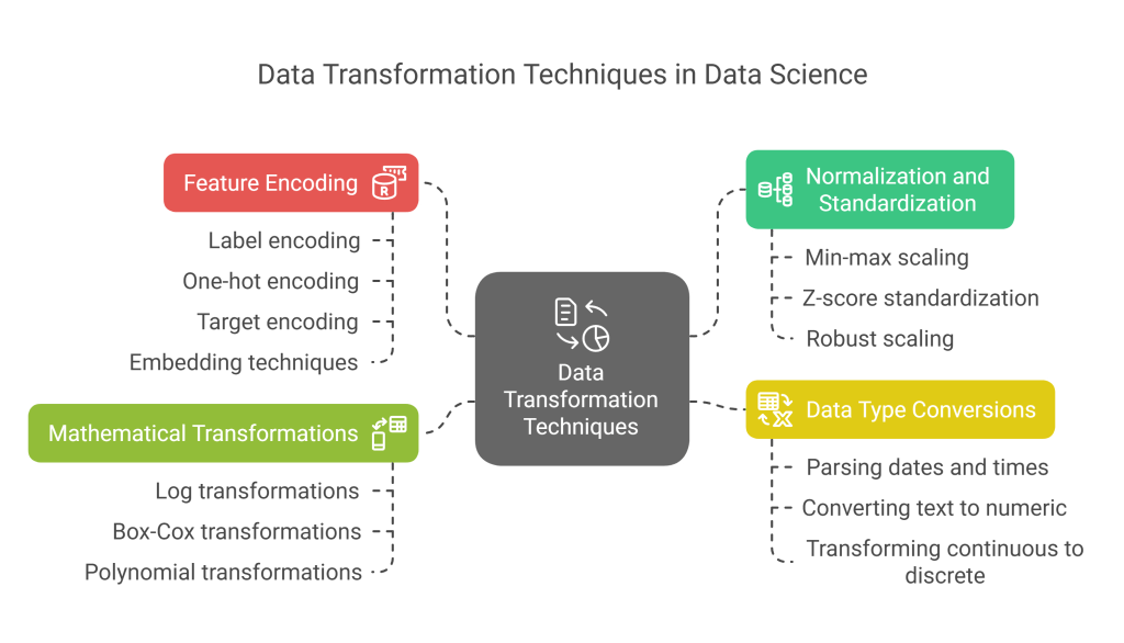
• Normalization and Standardization:
  • Min-max scaling: Rescaling features to a fixed range, typically [0,1]
  • Z-score standardization: Transforming data to have zero mean and unit variance
  • Robust scaling: Using statistics less sensitive to outliers, like median and IQR
• Feature Encoding:
  • Label encoding: Converting categorical variables to integers (appropriate for ordinal data)
  • One-hot encoding: Creating binary columns for each category (for nominal data)
  • Target encoding: Replacing categories with target statistics (e.g., mean target value per category)
  • Embedding techniques: Creating dense vector representations for high-cardinality categoricals
• Data Type Conversions:
  • Parsing dates and times into appropriate objects
  • Converting text to numeric data for analysis
  • Transforming continuous variables into discrete bins when appropriate
• Mathematical Transformations:
  • Log transformations for skewed distributions
  • Box-Cox or Yeo-Johnson transformations for normalizing data
  • Polynomial transformations for capturing non-linear relationships

These transformations should align with the assumptions of downstream modeling techniques and the nature of the data itself.

3.4 Feature Engineering

Feature engineering is the creative process of using domain knowledge to create new variables that better represent the underlying patterns:

• Feature Creation:
  • Interaction terms: Combining features to capture relationships (e.g., price × quantity)
  • Aggregate features: Summarizing grouped data (e.g., average purchase value per customer)
  • Time-based features: Extracting components from dates (day of week, month, seasons)
  • Domain-specific features: Creating variables based on business understanding
  • Text-derived features: Extracting information from textual data (sentiment, topics, etc.)
• Dimensionality Reduction:
  • Principal Component Analysis (PCA): Creating uncorrelated components that capture maximum variance
  • t-SNE and UMAP: Non-linear techniques for visualization and dimensionality reduction
  • Autoencoders: Neural network-based approach for finding efficient representations
• Feature Selection:
  • Filter methods: Using statistical measures like correlation or mutual information
  • Wrapper methods: Evaluating feature subsets using model performance
  • Embedded methods: Feature selection integrated into the modeling algorithm

Well-engineered features can significantly improve model performance by making patterns more explicit and reducing the complexity that the model needs to learn.

3.5 Handling Imbalanced Data

Many real-world datasets exhibit class imbalance, where some outcomes are much rarer than others. This imbalance can bias models toward the majority class, requiring special techniques:

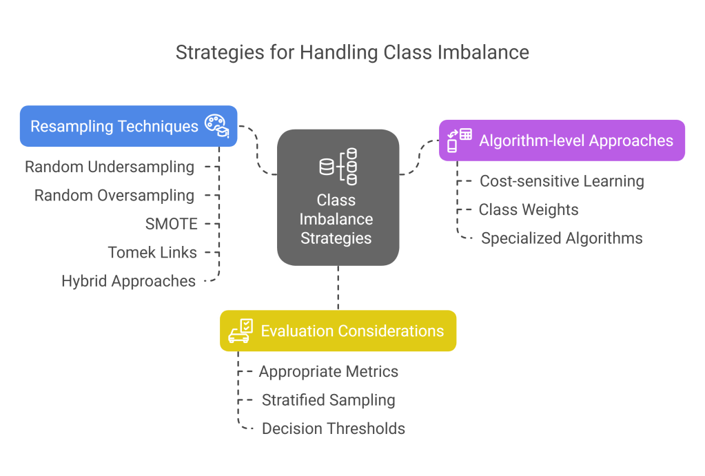
• Resampling Techniques:
  • Random undersampling: Reducing majority class observations
  • Random oversampling: Duplicating minority class observations
  • SMOTE (Synthetic Minority Over-sampling Technique): Generating synthetic minority class examples
  • Tomek links: Removing majority class examples near decision boundaries
  • Hybrid approaches: Combining undersampling and oversampling techniques
• Algorithm-level Approaches:
  • Cost-sensitive learning: Assigning higher misclassification costs to minority classes
  • Class weights: Adjusting the importance of each class during training
  • Specialized algorithms: Using methods designed for imbalanced data
• Evaluation Considerations:
  • Using appropriate metrics (precision, recall, F1-score, AUC) instead of accuracy
  • Stratified sampling to maintain class proportions in train/test splits
  • Performance evaluation across different decision thresholds

Data preparation is inherently iterative, often revisited as insights emerge during later phases. The decisions made during this phase profoundly influence model performance and the validity of conclusions drawn from the data.

Phase 4: Exploratory Data Analysis

Exploratory Data Analysis (EDA) is the critical process of investigating data patterns, detecting anomalies, testing hypotheses, and checking assumptions using statistical summaries and visualizations. EDA bridges data preparation and modeling by providing insights that inform feature engineering and model selection.

4.1 Statistical Summaries

Statistical summaries provide quantitative overviews of data distributions and relationships:

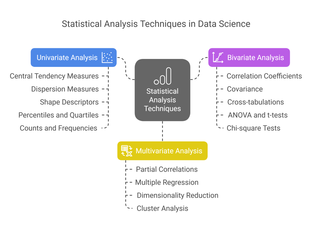
• Univariate Analysis:
  • Central tendency measures: mean, median, mode
  • Dispersion measures: standard deviation, variance, range, IQR
  • Shape descriptors: skewness, kurtosis
  • Percentiles and quartiles
  • Counts and frequencies for categorical variables
• Bivariate Analysis:
  • Correlation coefficients (Pearson, Spearman, Kendall)
  • Covariance
  • Cross-tabulations for categorical variables
  • ANOVA and t-tests for comparing groups
  • Chi-square tests for categorical associations
• Multivariate Analysis:
  • Partial correlations controlling for confounding variables
  • Multiple regression summaries
  • Dimensionality reduction techniques to identify patterns
  • Cluster analysis to identify natural groupings

Statistical summaries should be generated for both the overall dataset and meaningful segments to identify differences across groups and potential heterogeneity in relationships.

4.2 Data Visualization

Visualizations translate abstract data into accessible graphical representations that reveal patterns difficult to detect in raw numbers:

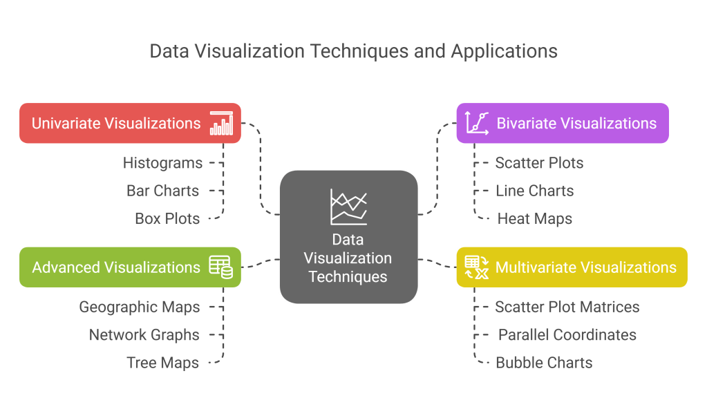
• Univariate Visualizations:
  • Histograms and density plots for continuous variables
  • Bar charts and pie charts for categorical variables
  • Box plots and violin plots for distribution details
  • QQ plots for comparing distributions to theoretical models
• Bivariate Visualizations:
  • Scatter plots for relationships between continuous variables
  • Line charts for time series or ordered data
  • Heat maps for correlation matrices
  • Grouped bar charts for categorical relationships
• Multivariate Visualizations:
  • Scatter plot matrices for multiple pairwise relationships
  • Parallel coordinates for high-dimensional data
  • Bubble charts adding a third dimension to scatter plots
  • Faceting and small multiples for comparing across categories
• Advanced Visualizations:
  • Geographic maps for spatial data
  • Network graphs for relationship data
  • Tree maps and sunburst diagrams for hierarchical data
  • Interactive visualizations allowing exploration of different dimensions

Effective visualizations simplify complexity, highlight key patterns, and communicate findings clearly. Tools like Matplotlib, Seaborn, Plotly, and Tableau enable sophisticated visualizations with relatively simple code.

4.3 Correlation Analysis

Correlation analysis systematically examines relationships between variables:

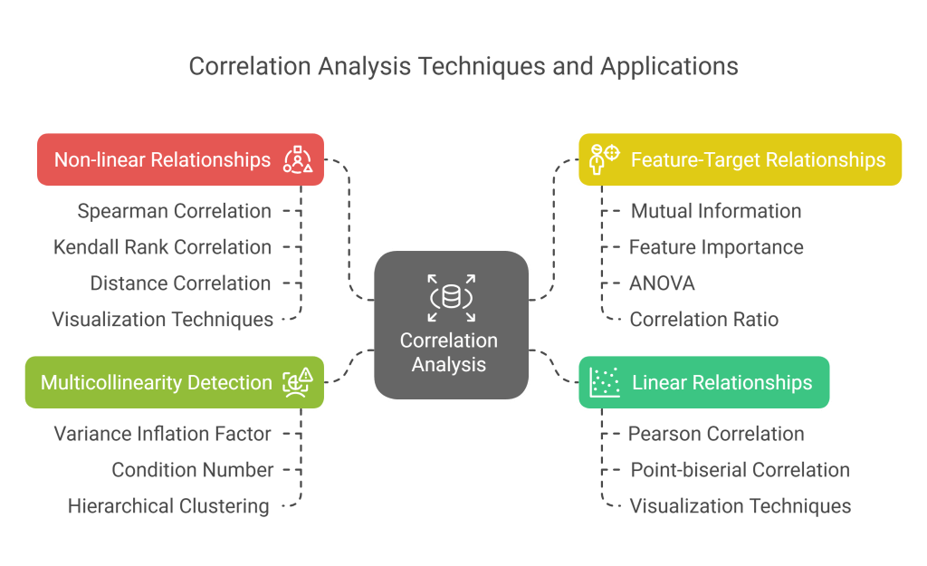
• Linear Relationships:
  • Pearson correlation for continuous variables
  • Point-biserial correlation between continuous and binary variables
  • Visualization using correlation heatmaps and scatter plots
• Non-linear Relationships:
  • Spearman and Kendall rank correlations for monotonic relationships
  • Distance correlation for detecting general statistical dependence
  • Visualization techniques like scatter plots with LOESS smoothing
• Feature-Target Relationships:
  • Mutual information for detecting non-linear associations with target
  • Feature importance from tree-based models
  • ANOVA for categorical predictors
  • Correlation ratio for non-linear relationships with categorical data
• Multicollinearity Detection:
  • Variance Inflation Factor (VIF) analysis
  • Condition number of the correlation matrix
  • Hierarchical clustering of the correlation matrix

Understanding correlations helps identify redundant features, suggests potential feature interactions, and reveals which variables might be most predictive of the target.

4.4 Hypothesis Generation

EDA is fundamentally about generating insights and hypotheses to guide further analysis:

• Pattern Identification:
  • Detecting trends in time series data
  • Identifying clusters or natural groupings
  • Recognizing seasonal or cyclical patterns
  • Observing differential effects across segments
• Anomaly Detection:
  • Spotting outliers and unusual patterns
  • Identifying data quality issues not caught during cleaning
  • Discovering unexpected relationships or behaviors
• Hypothesis Formulation:
  • Developing specific, testable hypotheses based on observed patterns
  • Prioritizing hypotheses based on potential business impact
  • Designing targeted analyses to validate or refute hypotheses
• Assumption Checking:
  • Verifying distributional assumptions for planned modeling approaches
  • Checking for linearity, homoscedasticity, or independence assumptions
  • Assessing whether data meets requirements for specific statistical tests

EDA should be documented thoroughly, with key visualizations, statistical findings, and generated hypotheses preserved for reference. This documentation guides feature engineering, helps communicate insights to stakeholders, and informs modeling decisions.

Ultimately, EDA is both science and art—combining rigorous statistical techniques with creative exploration to uncover hidden patterns and insights. It requires technical skills, domain knowledge, and curiosity to effectively navigate data complexities and extract meaningful understanding.

Phase 5: Data Modeling

Data modeling is the process of developing mathematical or computational structures that capture patterns in data and enable predictions or insights. This phase applies statistical and machine learning techniques to solve the business problem defined in earlier phases.

5.1 Selecting Modeling Techniques

The choice of modeling technique depends on the problem type, data characteristics, interpretability requirements, and computational constraints:

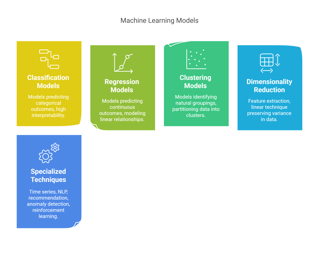
• Classification Models for predicting categorical outcomes:
  • Logistic Regression: Probabilistic approach with high interpretability
  • Decision Trees: Rule-based models with intuitive decision paths
  • Random Forests: Ensemble of trees with improved accuracy and stability
  • Gradient Boosting Machines: Sequential ensemble methods (XGBoost, LightGBM)
  • Support Vector Machines: Effective for high-dimensional spaces
  • Neural Networks: Deep learning approaches for complex patterns
  • Naive Bayes: Probabilistic approach based on Bayes’ theorem
• Regression Models for predicting continuous outcomes:
  • Linear Regression: Modeling linear relationships between variables
  • Polynomial Regression: Capturing non-linear patterns with polynomial terms
  • Ridge and Lasso Regression: Linear models with regularization
  • Decision Tree Regression: Non-parametric approach for complex relationships
  • Ensemble Regression Methods: Random forests and boosting for regression
  • Neural Network Regression: Deep learning for highly non-linear patterns
• Clustering Models for identifying natural groupings:
  • K-Means: Partitioning data into k clusters by minimizing within-cluster variance
  • Hierarchical Clustering: Building nested clusters without prespecifying count
  • DBSCAN: Density-based clustering for discovering arbitrary shapes
  • Gaussian Mixture Models: Probabilistic models assuming Gaussian distributions
  • Spectral Clustering: Using eigenvalues of similarity matrices for complex clusters
• Dimensionality Reduction for feature extraction:
  • Principal Component Analysis (PCA): Linear technique preserving variance
  • t-SNE: Non-linear technique preserving local similarities
  • UMAP: Manifold learning technique balancing local and global structure
  • Autoencoders: Neural network approach to unsupervised feature learning
• Specialized Techniques:
  • Time Series Models: ARIMA, Prophet, LSTM networks for sequential data
  • Natural Language Processing: Word embeddings, transformers for text
  • Recommendation Systems: Collaborative filtering, content-based methods
  • Anomaly Detection: Isolation forests, autoencoders, one-class SVM
  • Reinforcement Learning: For sequential decision-making problems

Selection criteria should include:

• Alignment with problem type (classification, regression, clustering)
• Performance expectations
• Interpretability requirements
• Training and inference time constraints
• Data volume and dimensionality
• Deployment environment limitations

5.2 Building Models

Model building implements selected techniques through a structured process:

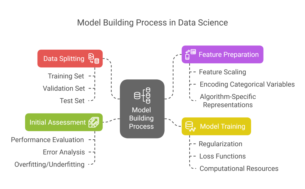
• Data Splitting:
  • Training set: For model fitting (typically 60-80% of data)
  • Validation set: For hyperparameter tuning (typically 10-20%)
  • Test set: For final evaluation (typically 10-20%)
  • Considerations for temporal data, grouped data, or imbalanced classes
• Feature Preparation:
  • Final transformations specific to the chosen algorithm
  • Feature scaling for distance-based algorithms
  • Encoding categorical variables appropriately
  • Creating algorithm-specific feature representations
• Model Training:
  • Fitting models to training data with appropriate parameters
  • Implementing regularization to prevent overfitting
  • Using appropriate loss functions for the problem
  • Managing computational resources for large datasets
  • Tracking training metrics and convergence
• Initial Assessment:
  • Evaluating performance on validation data
  • Analyzing prediction errors and patterns
  • Checking for signs of overfitting or underfitting
  • Comparing against baseline models

Multiple models should be built in parallel to enable comparison, starting with simpler models as baselines before moving to more complex approaches.

5.3 Model Assessment

Initial model assessment provides feedback for refinement:

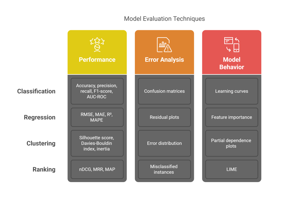
• Performance Metrics:
  • Classification: Accuracy, precision, recall, F1-score, AUC-ROC
  • Regression: RMSE, MAE, R², MAPE
  • Clustering: Silhouette score, Davies-Bouldin index, inertia
  • Ranking: nDCG, MRR, MAP
• Error Analysis:
  • Confusion matrices for classification models
  • Residual plots for regression models
  • Error distribution across different data segments
  • Identification of consistently misclassified instances
• Model Behavior Assessment:
  • Learning curves to diagnose bias-variance tradeoff
  • Feature importance analysis
  • Partial dependence plots for understanding feature effects
  • Local interpretable model-agnostic explanations (LIME)

This assessment informs model refinement and hyperparameter tuning decisions.

5.4 Hyperparameter Tuning

Hyperparameter tuning optimizes model configuration:

• Search Strategies:
  • Grid search: Exhaustive search across specified parameter values
  • Random search: Sampling parameter combinations randomly
  • Bayesian optimization: Using probabilistic models to select promising parameter sets
  • Evolutionary algorithms: Applying principles of natural selection to find optimal parameters
  • Gradient-based optimization: For differentiable hyperparameters
• Cross-Validation: Using techniques like k-fold cross-validation within the tuning process to ensure robust parameter selection.
• Automated Hyperparameter Tuning Tools: Leveraging libraries like Hyperopt, Optuna, or Scikit-Optimize to automate the search process.
• Tracking Experiments: Systematically logging parameter combinations and their corresponding performance to identify optimal settings and ensure reproducibility.

Effective hyperparameter tuning can significantly improve model performance by finding the configuration that best generalizes to unseen data.

5.5 Ensemble Methods

Ensemble methods combine multiple models to improve overall performance, stability, and robustness:

• Bagging (Bootstrap Aggregating):
  • Training multiple base models (e.g., decision trees) on different bootstrap samples of the training data.
  • Averaging predictions (for regression) or using majority voting (for classification).
  • Example: Random Forests.
• Boosting:
  • Sequentially training models, where each new model focuses on correcting errors made by previous models.
  • Assigning weights to training instances based on prediction difficulty.
  • Examples: AdaBoost, Gradient Boosting Machines (GBM), XGBoost, LightGBM, CatBoost.
• Stacking (Stacked Generalization):
  • Training multiple diverse base models.
  • Using a meta-model (or blender) to learn how to best combine the predictions of the base models.
  • Requires careful data splitting to avoid leakage.
• Voting:
  • Simple averaging or weighted averaging of predictions from multiple models (for regression).
  • Majority voting or weighted voting for classification.
• Benefits of Ensembles:
  • Often achieve higher accuracy than individual models.
  • Reduce variance and improve generalization.
  • More robust to noise and outliers.
• Considerations:
  • Increased computational cost and complexity.
  • Potentially reduced interpretability compared to simpler models.

Ensemble methods are a powerful tool in the data scientist’s arsenal, frequently leading to state-of-the-art results in various machine learning competitions and real-world applications.

Phase 6: Model Evaluation

Model evaluation is the rigorous process of assessing the performance, reliability, and business value of the trained models using unseen data. This phase determines whether a model is suitable for deployment and meets the project’s objectives.

6.1 Performance Metrics

Selecting appropriate performance metrics is crucial for evaluating models in the context of the business problem:

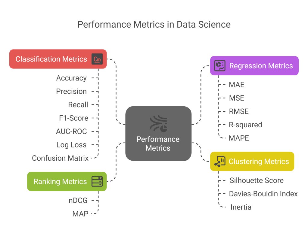
• Classification Metrics:
  • Accuracy: Proportion of correct predictions (can be misleading for imbalanced datasets).
  • Precision: Proportion of true positives among positive predictions (TP / (TP + FP)). Important when false positives are costly.
  • Recall (Sensitivity, True Positive Rate): Proportion of actual positives correctly identified (TP / (TP + FN)). Important when false negatives are costly.
  • F1-Score: Harmonic mean of precision and recall (2 * (Precision * Recall) / (Precision + Recall)). Balances precision and recall.
  • AUC-ROC (Area Under the Receiver Operating Characteristic Curve): Measures the model’s ability to distinguish between classes across all thresholds.
  • Log Loss (Cross-Entropy Loss): Penalizes confident incorrect predictions.
  • Confusion Matrix: Table showing true positives, true negatives, false positives, and false negatives.
• Regression Metrics:
  • Mean Absolute Error (MAE): Average absolute difference between predicted and actual values.
  • Mean Squared Error (MSE): Average squared difference; penalizes larger errors more.
  • Root Mean Squared Error (RMSE): Square root of MSE; in the same units as the target variable.
  • R-squared (Coefficient of Determination): Proportion of variance in the target variable explained by the model.
  • Mean Absolute Percentage Error (MAPE): Average percentage difference; useful for understanding error magnitude relative to actual values.
• Clustering Metrics:
  • Silhouette Score: Measures how similar an object is to its own cluster compared to other clusters.
  • Davies-Bouldin Index: Ratio of within-cluster scatter to between-cluster separation.
  • Inertia (Within-Cluster Sum of Squares): Sum of squared distances of samples to their closest cluster center (for K-Means).
• Ranking Metrics:
  • Normalized Discounted Cumulative Gain (nDCG): Evaluates ranking quality, considering the position and relevance of items.
  • Mean Average Precision (MAP): Average precision across multiple queries or users.The choice of metric should align with the specific business goals. For instance, in fraud detection, recall (catching as many fraudulent transactions as possible) might be prioritized over precision.

6.2 Cross-Validation Techniques

Cross-validation provides a more robust estimate of model performance and its ability to generalize to unseen data:

• K-Fold Cross-Validation:
  • Dataset is divided into k equal-sized folds.
  • Model is trained k times, each time using k-1 folds for training and the remaining fold for validation.
  • Performance metrics are averaged across the k iterations.
• Stratified K-Fold Cross-Validation: Ensures that each fold maintains approximately the same proportion of samples for each target class as in the complete dataset. Crucial for imbalanced datasets.
• Leave-One-Out Cross-Validation (LOOCV): A special case of k-fold where k equals the number of samples. Computationally expensive.
• Time Series Cross-Validation (Forward Chaining/Rolling Origin):
  • Maintains temporal order; trains on past data and validates on future data.
  • The training window can be fixed or expanding.
• Group K-Fold: Ensures that observations from the same group (e.g., same patient, same customer) are not split across training and validation sets to avoid data leakage.

Cross-validation helps in assessing model stability and provides a more reliable performance estimate than a single train-test split.

6.3 Model Comparison

Comparing multiple candidate models is essential to select the best performer:

• Baseline Models: Always compare against simple baselines (e.g., predicting the majority class, mean value, or a simple rule-based model) to demonstrate the value of more complex models.
• Statistical Significance Tests: Use tests like paired t-tests or McNemar’s test (for classification) to determine if performance differences between models are statistically significant.
• Performance vs. Complexity Trade-off: Consider Occam’s Razor – prefer simpler models if performance is comparable. Complex models can be harder to interpret, maintain, and deploy.
• Robustness Checks: Evaluate models on different data segments or under varying conditions to assess their stability.
• Business-Relevant Metrics: Beyond statistical metrics, evaluate models based on their potential business impact (e.g., cost savings, revenue increase).

A comprehensive comparison involves looking at various metrics, computational costs, interpretability, and alignment with deployment constraints.

6.4 Addressing Overfitting and Underfitting

• Overfitting (High Variance): Model performs well on training data but poorly on unseen data. It learns noise instead of the underlying signal.
  • Detection: Large gap between training and validation/test performance. Learning curves show training error decreasing while validation error plateaus or increases.
  • Solutions:
    • Get more training data.
    • Simplify the model (fewer features, less complex architecture).
    • Regularization (L1, L2, dropout).
    • Early stopping during training.
    • Cross-validation.
    • Feature selection.
• Underfitting (High Bias): Model performs poorly on both training and unseen data. It fails to capture the underlying patterns.
  • Detection: High training error and high validation/test error. Learning curves show both errors converging at a high level.
  • Solutions:
    • Use a more complex model.
    • Add more relevant features (feature engineering).
    • Reduce regularization.
    • Train for longer (if applicable).
    • Ensure data quality and relevance.

The goal is to find a model that balances bias and variance, achieving good generalization performance on new, unseen data.

Phase 7: Model Deployment

Model deployment is the process of integrating a trained and evaluated machine learning model into a production environment where it can make predictions on new data and deliver business value.

7.1 Deployment Planning

Careful planning is essential for a smooth deployment:

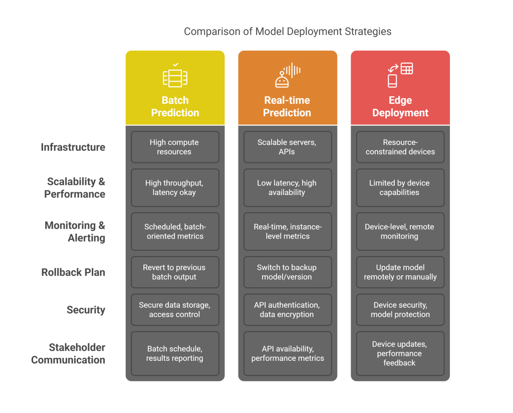
• Deployment Strategy:
  • Batch Prediction: Model makes predictions on a batch of data at scheduled intervals.
  • Real-time Prediction (Online Inference): Model provides predictions on demand for individual instances, often via an API.
  • Edge Deployment: Model runs directly on devices (e.g., mobile phones, IoT sensors).
• Infrastructure Requirements: Determine necessary hardware (CPU, GPU, memory), software dependencies, and network configurations.
• Scalability and Performance: Plan for expected load, latency requirements, and throughput.
• Monitoring and Alerting: Define how model performance, system health, and data drift will be tracked.
• Rollback Plan: Have a strategy to revert to a previous model version or a safe state if issues arise.
• Security Considerations: Address data privacy, model security, and access control.
• Stakeholder Communication: Keep relevant teams (IT, operations, business users) informed about the deployment schedule and potential impacts.

7.2 Implementation Strategies

Various approaches can be used to make the model accessible:

• Model as an API: Exposing the model’s prediction functionality via a REST API (e.g., using Flask, FastAPI, or serverless functions). This is common for real-time inference.
• Embedding in Applications: Integrating the model directly into existing software applications.
• Batch Scoring Systems: Setting up scheduled jobs (e.g., using Airflow, cron) to run the model on new batches of data and store predictions.
• Containerization (Docker, Kubernetes): Packaging the model and its dependencies into containers for portability, scalability, and easier management.
• Cloud ML Platforms: Leveraging services like AWS SageMaker, Google AI Platform, or Azure Machine Learning for streamlined deployment and management.
• Shadow Deployment (Dark Launch): Deploying the new model alongside the existing one to monitor its predictions without affecting live traffic, allowing for comparison and validation.
• Canary Releases/Blue-Green Deployment: Gradually rolling out the new model to a subset of users or traffic before a full switchover.

7.3 Integration with Existing Systems

The deployed model needs to interact with other components of the business infrastructure:

• Data Pipelines: Connecting the model to live data sources for input and ensuring predictions are delivered to downstream systems (e.g., databases, dashboards, applications).
• Upstream Systems: Ensuring data quality and format consistency from sources providing input to the model.
• Downstream Consumers: Making predictions available in a usable format for applications, reporting tools, or decision-making processes.
• Authentication and Authorization: Implementing security measures to control access to the model and its predictions.
• Logging and Auditing: Recording prediction requests, responses, and any errors for debugging and compliance.

7.4 Monitoring and Maintenance

Once deployed, models require ongoing monitoring and maintenance to ensure continued performance and relevance:

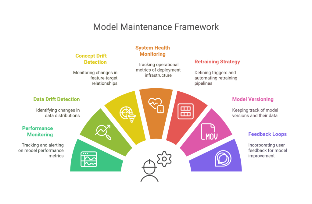
• Performance Monitoring:
  • Tracking key model metrics (accuracy, precision, recall, RMSE, etc.) on live data.
  • Setting up alerts for significant performance degradation.
• Data Drift Detection:
  • Monitoring the statistical properties of input data over time.
  • Detecting changes in data distributions that could invalidate the model (e.g., new categories, shifted numerical ranges).
• Concept Drift Detection:
  • Monitoring changes in the underlying relationship between input features and the target variable.
  • The patterns the model learned may no longer hold true.
• System Health Monitoring: Tracking CPU usage, memory, latency, error rates, and other operational metrics of the deployment infrastructure.
• Retraining Strategy:
  • Defining triggers for model retraining (e.g., performance drop, significant data/concept drift, scheduled intervals).
  • Automating the retraining pipeline where possible.
• Model Versioning: Keeping track of different model versions, their training data, and performance for reproducibility and rollback.
• Feedback Loops: Incorporating feedback from users and downstream systems to identify areas for improvement or retraining.

Effective monitoring and maintenance are crucial for the long-term success and value of a deployed machine learning model, forming a key part of MLOps (Machine Learning Operations).

Phase 8: Communication and Visualization

Communicating insights effectively to diverse audiences is as crucial as the technical aspects of data science. This phase focuses on translating complex findings into understandable and actionable information.

8.1 Storytelling with Data

Data storytelling involves weaving a compelling narrative around data insights to engage and persuade stakeholders:

• Identify the Audience: Tailor the story to their background, interests, and level of technical understanding.
• Define the Key Message: What is the single most important insight you want to convey?
• Structure the Narrative:
  • Setup: Provide context and define the problem or question.
  • Conflict/Challenge: Describe the analysis and the patterns or obstacles encountered.
  • Resolution: Present the key findings and their implications.
  • Call to Action: Suggest recommendations or next steps.
• Use Visuals Effectively: Support the narrative with clear and impactful visualizations.
• Keep it Concise and Focused: Avoid overwhelming the audience with too much information.
• Emphasize Business Impact: Connect insights to tangible business outcomes.

8.2 Creating Effective Visualizations

Visualizations are powerful tools for communication, but they must be designed thoughtfully:

• Choose the Right Chart Type: Select charts that best represent the data and the message (e.g., bar charts for comparisons, line charts for trends, scatter plots for relationships, maps for geospatial data).
• Clarity and Simplicity: Avoid clutter, unnecessary decorations (“chart junk”), and misleading scales.
• Accurate Representation: Ensure visuals faithfully represent the data without distortion.
• Labeling and Annotation: Use clear titles, axis labels, legends, and annotations to explain key elements.
• Color Choices: Use color purposefully to highlight patterns or categories, ensuring accessibility (e.g., colorblind-friendly palettes).
• Context is Key: Provide enough context for the audience to understand what the visualization shows and why it matters.
• Interactivity (When Appropriate): Interactive dashboards (e.g., using Tableau, Power BI, Plotly Dash) can allow users to explore data themselves.

8.3 Presenting to Different Audiences

The style and content of communication should vary based on the audience:

• Technical Audiences (e.g., other data scientists, engineers):
  • Can delve into methodological details, model specifics, and statistical rigor.
  • May appreciate discussions of limitations, assumptions, and alternative approaches.
• Business Stakeholders (e.g., executives, managers):
  • Focus on high-level insights, business implications, and actionable recommendations.
  • Use clear, non-technical language and compelling visuals.
  • Emphasize ROI, strategic alignment, and decision support.
• General Audiences:
  • Simplify complex concepts and avoid jargon.
  • Use relatable examples and focus on the “so what?” of the findings.

Regardless of the audience, be prepared to answer questions and engage in discussion.

8.4 Actionable Insights

The ultimate goal of data science is to drive action and create value. Insights are actionable when they:

• Are Clear and Understandable: Easily grasped by the intended audience.
• Are Relevant to Business Objectives: Directly address the problems or opportunities defined earlier.
• Provide Specific Recommendations: Suggest concrete steps that can be taken based on the findings.
• Are Supported by Evidence: Backed by robust data analysis and model results.
• Consider Constraints and Feasibility: Take into account practical limitations and resources.
• Quantify Potential Impact: Estimate the benefits or outcomes of implementing the recommendations.

Effective communication transforms data-driven findings into tangible business improvements and strategic decisions.

Advanced Data Science Techniques

This section delves into specific techniques that are often employed during various phases of the data science life cycle, particularly in data preparation and modeling.

11.1 Vector Embeddings

Vector embeddings are dense, low-dimensional representations of discrete or high-dimensional data, such as words, sentences, documents, users, products, or nodes in a graph.

• Purpose: To capture semantic relationships and contextual information in a way that machine learning models can easily process. Similar items are represented by vectors that are close together in the embedding space.
• Applications:

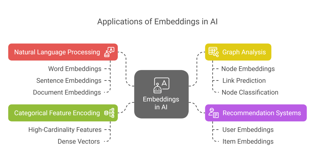
• Natural Language Processing (NLP): Word embeddings (e.g., Word2Vec, GloVe, FastText), sentence embeddings (e.g., Sentence-BERT), document embeddings. Used for tasks like text classification, sentiment analysis, machine translation, and information retrieval.
• Recommendation Systems: Embedding users and items to predict preferences and make recommendations.
• Graph Analysis: Node embeddings (e.g., Node2Vec, DeepWalk) to capture graph structure for link prediction or node classification.
• Categorical Feature Encoding: Representing high-cardinality categorical features as dense vectors.
• How they work (General Idea):
  • Often learned using neural networks.
  • The network is trained on a related task (e.g., predicting a word from its context for word embeddings).
  • The weights of a hidden layer in the network then serve as the embedding for the input.
• Benefits:
  • Reduce dimensionality while preserving meaningful relationships.
  • Improve model performance by providing richer feature representations.
  • Enable similarity calculations and analogies (e.g., “king – man + woman = queen” with word embeddings).

11.2 One-Hot Encoding

One-hot encoding is a common technique used to convert categorical string or integer data into a numerical format that can be fed into machine learning algorithms.

• Purpose: To represent categorical variables without imposing an artificial ordinal relationship between categories.
• How it works:
• For a categorical feature with ‘N’ unique categories, one-hot encoding creates ‘N’ new binary (0 or 1) features.
• Each new feature corresponds to one unique category.
• For a given data point, the binary feature corresponding to its category is set to 1, and all other binary features are set to 0.
• Example:
  • Categorical Feature: “Color” with categories {“Red”, “Green”, “Blue”}
  • One-Hot Encoded Features: “Is_Red”, “Is_Green”, “Is_Blue”
  • If a data point has Color = “Green”, its encoded representation would be: Is_Red=0, Is_Green=1, Is_Blue=0.
• Advantages:
  • Prevents models from assuming an incorrect order or ranking among categories (unlike label encoding for nominal data).
  • Many machine learning algorithms (e.g., linear models, neural networks) work better with this representation.
• Disadvantages:
  • Can lead to a high number of features if the categorical variable has many unique categories (high cardinality), which can increase computational cost and potentially lead to the “curse of dimensionality.”
  • For tree-based models, one-hot encoding might not always be necessary or optimal.
• Considerations:
  • For very high cardinality features, other encoding methods (e.g., target encoding, embedding, or grouping rare categories) might be more appropriate.
  • Be careful about multicollinearity (dummy variable trap) if all N binary features are used; often, N-1 features are used, and the Nth category is implicitly represented.

11.3 SMOTE for Imbalanced Data

SMOTE (Synthetic Minority Over-sampling Technique) is an oversampling method used to address class imbalance in datasets where one class (the minority class) is significantly underrepresented compared to another class (the majority class).

• Purpose: To balance the class distribution by creating synthetic samples of the minority class, thereby helping machine learning models learn to identify the minority class more effectively.
• How it works:
  1. For each instance in the minority class, SMOTE finds its ‘k’ nearest neighbors (also from the minority class).
  2. It then randomly selects one of these neighbors.
  3. A synthetic instance is created by interpolating between the original instance and the selected neighbor along the line segment joining them in the feature space.
  • The amount of oversampling (number of synthetic samples to create) is typically a parameter.
• Advantages:
  • Helps mitigate the bias of models towards the majority class.
  • Can improve the recall and F1-score for the minority class.
  • Generates new, plausible minority samples rather than just duplicating existing ones (like random oversampling).
• Disadvantages and Considerations:
  • Can generate noisy samples if the minority class is sparse or overlaps significantly with the majority class.
  • May not be effective for very high-dimensional data.
  • Variants of SMOTE (e.g., Borderline-SMOTE, ADASYN) have been developed to address some of these limitations by focusing on samples near the decision boundary or those that are harder to learn.
  • SMOTE should typically be applied only to the training data, not the validation or test data, to avoid data leakage and get a realistic estimate of model performance.
  • It’s often beneficial to combine SMOTE with undersampling techniques for the majority class.

11.4 Feature Selection Methods

Feature selection is the process of identifying and selecting a subset of relevant features from the original set of features to use in model building.

• Purpose:
  • Improve model performance by removing irrelevant or redundant features.
  • Reduce model complexity and training time.
  • Enhance model interpretability.
  • Avoid the curse of dimensionality.
• Types of Feature Selection Methods:
  1. Filter Methods:
     • Evaluate features based on their intrinsic statistical properties (e.g., correlation with the target, mutual information, chi-squared test, ANOVA F-value) independently of any machine learning algorithm.
     • Fast and computationally inexpensive.
     • May not select the optimal feature subset for a specific model.
  2. Wrapper Methods:
     • Use a specific machine learning algorithm to evaluate the usefulness of feature subsets.
     • Treat the feature selection process as a search problem, where different subsets are generated and evaluated by training and testing the model.
     • Examples: Recursive Feature Elimination (RFE), Forward Selection, Backward Elimination.
     • Computationally more expensive but can lead to better model-specific feature sets.
  3. Embedded Methods:
     • Perform feature selection as part of the model training process itself.
     • The algorithm inherently selects or assigns weights to features.
     • Examples: LASSO (L1 regularization) which shrinks coefficients of less important features to zero, tree-based models (like Random Forest or Gradient Boosting) which provide feature importance scores.
     • Often offer a good balance between performance and computational cost.
• Considerations:
  • The choice of method depends on the dataset size, number of features, type of data, and the chosen modeling algorithm.
  • It’s crucial to perform feature selection using only the training data to avoid data leakage from the validation or test sets.
  • Domain knowledge can also play a vital role in guiding feature selection.

Ethics and Responsible Data Science

As data science becomes more powerful and pervasive, it’s crucial to address the ethical implications and ensure that its applications are responsible, fair, and transparent.

12.1 Privacy Considerations

Data science often relies on large datasets, which may contain sensitive personal information.

• Data Minimization: Collect and retain only the data that is strictly necessary for the intended purpose.
• Anonymization and Pseudonymization:
  • Anonymization: Removing or altering personally identifiable information (PII) so that individuals cannot be re-identified. This is often difficult to achieve perfectly.
  • Pseudonymization: Replacing PII with artificial identifiers (pseudonyms). The original identifiers are kept separate and secure, allowing for re-identification if necessary (e.g., for data correction) but protecting privacy during analysis.
• Differential Privacy: A formal mathematical framework that adds noise to data or query results to protect individual privacy while still allowing for useful aggregate analysis.
• Secure Data Handling: Implementing robust security measures for data storage, access, and transmission to prevent unauthorized access or breaches.
• Compliance with Regulations: Adhering to data privacy laws like GDPR (General Data Protection Regulation) in Europe, CCPA (California Consumer Privacy Act), HIPAA (for healthcare data in the US), etc. This includes obtaining consent, providing data access rights, and ensuring data portability.
• Privacy-Preserving Machine Learning: Developing techniques that allow models to be trained on data without exposing the raw individual data points (e.g., federated learning, homomorphic encryption).

12.2 Bias and Fairness

Machine learning models can inadvertently learn and perpetuate existing societal biases present in the data they are trained on, leading to unfair or discriminatory outcomes.

• Sources of Bias:
  • Historical Bias: Data reflects past prejudices (e.g., gender or racial bias in hiring).
  • Representation Bias: Certain groups are underrepresented or overrepresented in the data.
  • Measurement Bias: Features or labels are measured or collected differently across groups.
  • Algorithmic Bias: The algorithm itself, or how it’s optimized, can introduce bias.
• Defining Fairness: Fairness is a complex, context-dependent concept with multiple mathematical definitions (e.g., demographic parity, equalized odds, equal opportunity). The appropriate definition depends on the application and societal values.
• Bias Detection Techniques:
  • Auditing datasets for representation disparities.
  • Evaluating model performance metrics (e.g., accuracy, false positive/negative rates) separately for different demographic groups.
• Bias Mitigation Strategies:
  • Pre-processing: Modifying the training data (e.g., re-weighting, resampling, fair synthetic data generation).
  • In-processing: Modifying the learning algorithm or adding fairness constraints during training.
  • Post-processing: Adjusting model predictions to satisfy fairness criteria.
• Fairness Audits: Regularly assessing models for biased outcomes and taking corrective action.

12.3 Transparency and Explainability

Many advanced machine learning models, especially deep learning models, operate as “black boxes,” making it difficult to understand how they arrive at their predictions.

• Importance of Explainability (XAI – Explainable AI):
  • Trust and Accountability: Users and stakeholders are more likely to trust and adopt models if they understand their reasoning.
  • Debugging and Improvement: Understanding why a model makes errors can help improve it.
  • Regulatory Compliance: Some regulations may require explanations for automated decisions.
  • Fairness Assessment: Explanations can help identify if a model is relying on biased features.
• Techniques for Explainability:
  • Model-Agnostic Methods: Can be applied to any model (e.g., LIME – Local Interpretable Model-agnostic Explanations, SHAP – SHapley Additive exPlanations). These methods explain individual predictions by showing feature contributions.
  • Model-Specific Methods: Techniques tailored to specific model types (e.g., feature importance from tree-based models, activation maps in neural networks).
  • Interpretable Models: Using inherently simpler and more transparent models like linear regression, logistic regression, or decision trees when possible.
• Transparency in Process: Documenting the data sources, preprocessing steps, model choices, and evaluation criteria.

12.4 Ethical Guidelines

Establishing and adhering to ethical guidelines is fundamental for responsible data science.

• Beneficence and Non-Maleficence: Striving to create solutions that benefit society and actively avoiding harm.
• Accountability and Responsibility: Data scientists and organizations are responsible for the impact of their models and systems.
• Human Oversight: Ensuring that automated decisions can be reviewed and overridden by humans, especially in critical applications.
• Ethical Review Boards: Establishing internal or external bodies to review data science projects for ethical implications.
• Professional Codes of Conduct: Following guidelines from professional organizations (e.g., ACM Code of Ethics).
• Continuous Learning and Dialogue: Staying informed about emerging ethical challenges and engaging in discussions about responsible AI.

Responsible data science requires a proactive and ongoing commitment to these principles throughout the entire data science life cycle.

Case Studies

Illustrating the data science life cycle with real-world examples can provide practical context.

13.1 Predictive Maintenance in Manufacturing

• Business Objective: Reduce unplanned downtime and maintenance costs by predicting when industrial machinery is likely to fail.
• Data Acquisition: Sensor data from machines (temperature, pressure, vibration, RPM), historical maintenance logs, machine specifications, operational parameters.
• Data Preparation: Cleaning sensor noise, handling missing data, synchronizing time-series data, feature engineering (e.g., rolling averages, Fourier transforms of vibration data, time since last maintenance).
• Exploratory Data Analysis: Visualizing sensor trends leading up to failures, correlating sensor readings with failure events.
• Data Modeling: Using classification models (e.g., Random Forest, LSTM networks) to predict failure within a specific future window (e.g., next 24 hours) or regression models to predict Remaining Useful Life (RUL).
• Model Evaluation: Metrics like precision, recall (for failure prediction), F1-score, and RMSE (for RUL). Cost-based evaluation considering the cost of false positives (unnecessary maintenance) vs. false negatives (unplanned downtime).
• Model Deployment: Integrating the model with a monitoring system that alerts maintenance teams about impending failures. This could be real-time alerts or batch predictions.
• Communication: Presenting findings to plant managers and maintenance engineers, demonstrating potential cost savings and operational improvements.

13.2 Customer Churn Prediction

• Business Objective: Reduce customer attrition by identifying customers at high risk of churning and implementing targeted retention strategies.
• Data Acquisition: Customer demographics, purchase history, website/app usage logs, customer service interactions, subscription details, marketing responses.
• Data Preparation: Handling missing values, encoding categorical features (e.g., subscription plan), feature engineering (e.g., recency, frequency, monetary value (RFM), average session duration, number of support tickets).
• Exploratory Data Analysis: Identifying patterns in churned vs. active customers, visualizing feature distributions for different segments.
• Data Modeling: Using classification models (e.g., Logistic Regression, Gradient Boosting, Neural Networks) to predict the probability of a customer churning within a defined period.
• Model Evaluation: Metrics like AUC-ROC, precision, recall (to catch potential churners), lift charts, and profit curves (to assess business impact of retention campaigns).
• Model Deployment: Integrating the model with CRM systems to flag at-risk customers, enabling marketing or customer service teams to take proactive retention actions (e.g., targeted offers, support outreach).
• Communication: Explaining churn drivers to marketing and sales teams, demonstrating the ROI of retention efforts.

13.3 Healthcare Diagnosis Assistance

• Business Objective: Assist medical professionals in making faster and more accurate diagnoses, for example, by identifying cancerous cells in medical images or predicting disease risk based on patient data.
• Data Acquisition: Medical images (X-rays, MRIs, CT scans), electronic health records (EHRs), genomic data, patient-reported outcomes, lab results.
• Data Preparation: Image preprocessing (normalization, augmentation), cleaning and standardizing EHR data, handling missing values, feature engineering (e.g., extracting features from images using CNNs, creating risk scores from patient history).
• Exploratory Data Analysis: Visualizing image features, identifying correlations between patient characteristics and disease prevalence.
• Data Modeling:
  • For image analysis: Convolutional Neural Networks (CNNs) for image classification or segmentation.
  • For risk prediction: Classification models (e.g., SVM, Random Forest) using structured patient data.
• Model Evaluation: Metrics like sensitivity (recall), specificity, precision, F1-score, AUC-ROC. Crucially, considering the clinical significance of false positives and false negatives. Rigorous validation against expert diagnoses.
• Model Deployment: Integrating the model into clinical decision support systems or diagnostic tools. Requires careful consideration of regulatory approvals (e.g., FDA), usability by clinicians, and integration with hospital IT systems. The model serves as an aid, not a replacement for human expertise.
• Communication: Presenting model performance and limitations to clinicians, researchers, and regulatory bodies, emphasizing its role in augmenting human decision-making.

Industry-Specific Considerations

The application and nuances of the data science life cycle can vary significantly across different industries due to unique data types, regulatory environments, business objectives, and ethical challenges.

14.1 Healthcare

• Data Sources: Electronic Health Records (EHRs), medical imaging (X-rays, MRIs), genomic sequences, wearable sensor data, clinical trial data, insurance claims.
• Key Challenges:
  • Data Privacy and Security: Strict regulations like HIPAA.
  • Data Silos and Interoperability: Data often fragmented across different systems.
  • Complex and Heterogeneous Data: Combining structured, unstructured (clinical notes), and image data.
  • Interpretability and Explainability: Crucial for clinical adoption and trust.
  • Bias and Fairness: Ensuring models don’t exacerbate health disparities.
• Applications: Disease diagnosis and prediction, drug discovery, personalized medicine, patient risk stratification, hospital operations optimization, fraud detection in claims.
• Ethical Focus: Patient consent, avoiding harm, ensuring equitable access to benefits of AI.

14.2 Finance and Banking

• Data Sources: Transaction records, credit scores, market data, customer profiles, news articles, social media sentiment.
• Key Challenges:
  • Regulatory Compliance: Strict oversight (e.g., Basel accords, anti-money laundering laws).
  • Fraud Detection: Adversarial attacks and evolving fraud patterns.
  • Model Risk Management: Ensuring model robustness and stability, especially for high-stakes decisions.
  • Real-time Processing: Need for low-latency predictions (e.g., algorithmic trading, fraud alerts).
  • Explainability: Required for regulatory audits and customer trust (e.g., loan application decisions).
• Applications: Algorithmic trading, credit scoring, fraud detection, risk management, customer segmentation, personalized financial advice, anti-money laundering (AML).
• Ethical Focus: Fairness in lending, preventing discriminatory practices, market stability.

14.3 Retail and E-commerce

• Data Sources: Point-of-sale (POS) data, online browsing history, purchase history, customer reviews, loyalty program data, social media trends, supply chain information.
• Key Challenges:
  • Scalability: Handling large volumes of customer and transaction data.
  • Personalization vs. Privacy: Balancing targeted marketing with customer privacy concerns.
  • Dynamic Pricing: Optimizing prices in real-time based on demand and competition.
  • Inventory Management: Predicting demand to optimize stock levels.
• Applications: Recommendation systems, customer segmentation and targeting, demand forecasting, price optimization, supply chain optimization, churn prediction, sentiment analysis of reviews.
• Ethical Focus: Transparency in pricing and recommendations, data usage consent.

14.4 Manufacturing (Industry 4.0)

• Data Sources: IoT sensor data from machinery (temperature, vibration, pressure), production line data (output, defects), supply chain data, maintenance logs, quality control records.
• Key Challenges:
  • Data Volume and Velocity: Streaming data from numerous sensors.
  • Integration of OT and IT Data: Combining operational technology data with enterprise IT systems.
  • Predictive Maintenance: Accurately forecasting equipment failures.
  • Quality Control: Automating defect detection.
• Applications: Predictive maintenance, quality control and anomaly detection, production process optimization, supply chain visibility, demand forecasting, energy consumption optimization.
• Ethical Focus: Worker displacement due to automation, safety of AI-controlled systems.

Future Trends in Data Science

The field of data science is rapidly evolving, driven by advancements in algorithms, computing power, and data availability. Several key trends are shaping its future:

15.1 AutoML (Automated Machine Learning)

• Concept: Automating the end-to-end process of applying machine learning to real-world problems, including data preparation, feature engineering, model selection, hyperparameter tuning, and model deployment.
• Goal: To make machine learning more accessible to non-experts (democratization of AI) and to improve the efficiency and productivity of data scientists by automating repetitive tasks.
• Tools and Platforms: Google AutoML, H2O.ai, Auto-sklearn, TPOT.
• Impact: Allows for faster model development and iteration, potentially leading to better-performing models by exploring a wider range of possibilities than manual efforts might cover. However, domain expertise remains crucial for problem formulation and result interpretation.

15.2 MLOps (Machine Learning Operations)

• Concept: A set of practices that aims to deploy and maintain machine learning models in production reliably and efficiently. It combines ML, DevOps, and Data Engineering principles.
• Focus Areas: Model versioning, continuous integration/continuous deployment (CI/CD) for ML pipelines, automated retraining, model monitoring (for performance, data drift, concept drift), infrastructure management, and governance.
• Goal: To streamline the ML lifecycle, reduce time to deployment, ensure model quality and reliability in production, and facilitate collaboration between data scientists, ML engineers, and operations teams.
• Impact: Essential for scaling ML applications and realizing sustained business value from data science initiatives.

15.3 Edge AI

• Concept: Running AI algorithms directly on edge devices (e.g., smartphones, IoT sensors, autonomous vehicles, industrial robots) rather than in centralized cloud environments.
• Drivers: Need for low latency, reduced bandwidth consumption, improved privacy (data stays local), and offline operation.
• Techniques: Model compression (e.g., quantization, pruning), efficient neural network architectures (e.g., MobileNets), specialized AI hardware for edge devices (e.g., NPUs, TPUs).
• Applications: Real-time object detection in autonomous vehicles, voice assistants on smart speakers, predictive maintenance on factory equipment, smart healthcare monitoring.
• Impact: Enables new classes of AI applications that require immediate processing and local intelligence.

15.4 Federated Learning

• Concept: A machine learning technique that trains a shared global model across many decentralized edge devices or servers holding local data samples, without exchanging the local data itself.
• How it works:
  1. A central server sends the current global model to participating devices.
  2. Each device trains the model on its local data.
  3. Devices send their updated model parameters (not the data) back to the server.
  4. The server aggregates these parameters (e.g., by averaging) to create an improved global model. This process is repeated.
• Benefits:
  • Privacy Preservation: Raw data remains on the local device.
  • Reduced Communication Costs: Only model updates are transmitted.
  • Leverages Distributed Data: Enables learning from diverse datasets without centralizing them.
• Applications: Improving keyboard predictions on smartphones, personalized recommendations, healthcare research across hospitals without sharing patient records.
• Impact: Addresses critical privacy concerns and enables collaborative model building on sensitive, distributed datasets.

Conclusion

The data science life cycle provides a structured and iterative framework for transforming raw data into actionable insights and valuable solutions. From clearly defining business objectives and meticulously acquiring and preparing data, through insightful exploratory analysis and robust modeling, to rigorous evaluation and effective deployment, each phase plays a critical role in the success of a data science project. The journey doesn’t end with deployment; continuous monitoring, communication of results, and adherence to ethical principles are paramount for sustained impact and responsible innovation.

As we’ve seen, specialized techniques like vector embeddings, one-hot encoding, and SMOTE enhance our ability to process diverse data types and tackle complex challenges like imbalanced datasets. Furthermore, the ethical dimensions of data science—privacy, fairness, transparency, and accountability—are not mere afterthoughts but integral components that must be woven into every stage of the life cycle.

The applications of data science are vast and continue to expand across industries, driving efficiency, personalization, and discovery. With emerging trends like AutoML, MLOps, Edge AI, and Federated Learning, the field is poised for even greater advancements, making data science an increasingly powerful and accessible tool for organizations and society. By understanding and mastering the comprehensive data science life cycle, practitioners and leaders can unlock the full potential of data to solve meaningful problems and shape a data-driven future.