When you build a machine learning model to classify data—whether it’s identifying spam emails, detecting fraudulent transactions, or diagnosing diseases—how do you know if it’s actually doing a good job? Simply building a model isn’t enough; you need to evaluate its performance. This is where classification metrics come into play. They provide a quantitative way to assess how well your model is performing and help you compare different models.

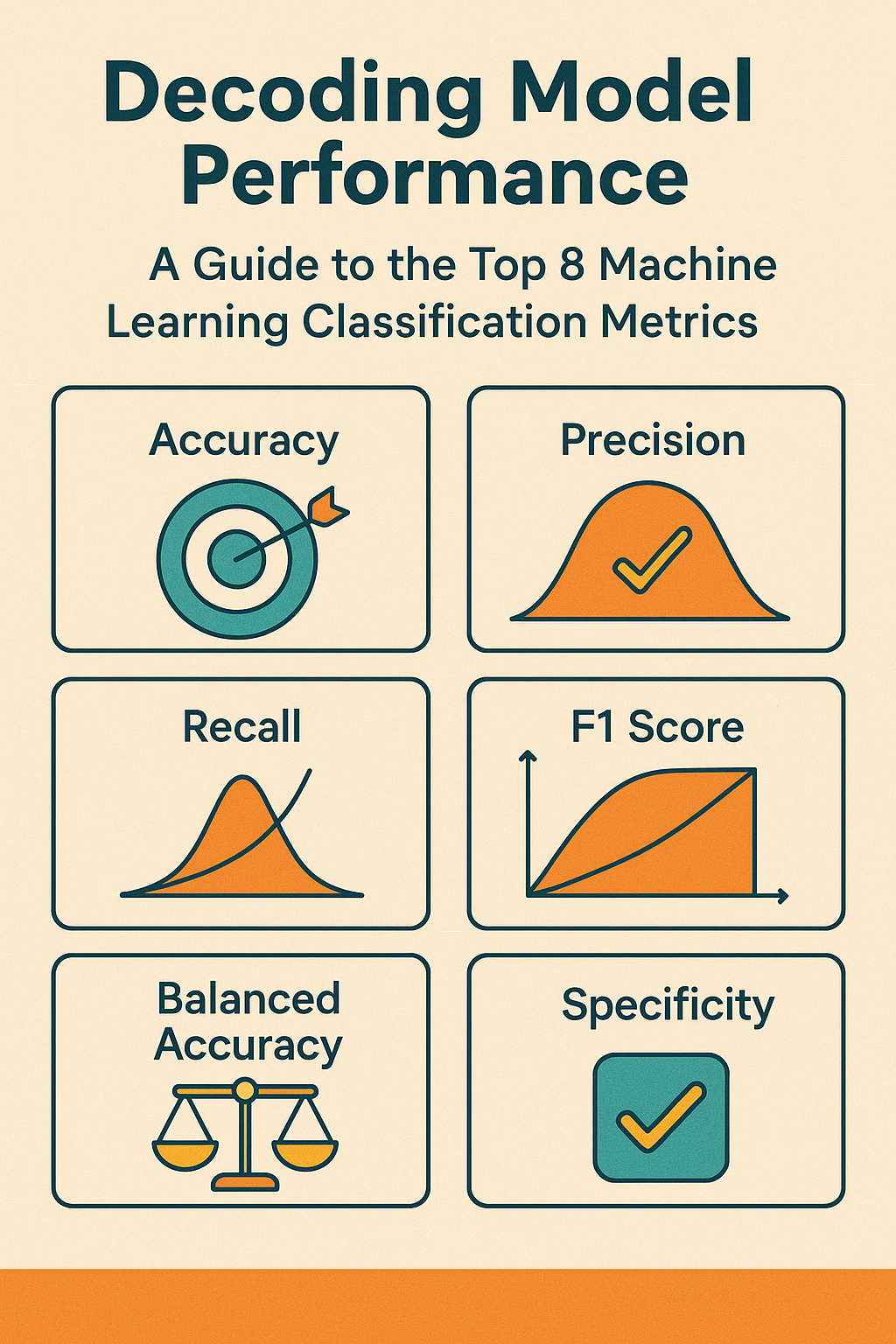
Let’s dive into eight of the most common and crucial classification metrics that every data scientist and machine learning enthusiast should understand.

Before we jump into the metrics, let’s quickly define some common terms used in their formulas:

• True Positives (TP): The number of positive instances correctly classified as positive. (e.g., correctly identifying a spam email as spam).
• True Negatives (TN): The number of negative instances correctly classified as negative. (e.g., correctly identifying a non-spam email as not spam).
• False Positives (FP): The number of negative instances incorrectly classified as positive. Also known as a “Type I error.” (e.g., incorrectly identifying a non-spam email as spam).
• False Negatives (FN): The number of positive instances incorrectly classified as negative. Also known as a “Type II error.” (e.g., incorrectly identifying a spam email as not spam).

Now, let’s explore the metrics!

1. Accuracy

Formula:Accuracy=TP+TN+FP+FNTP+TN​

What it is: Accuracy is perhaps the most intuitive metric. It measures the proportion of total predictions that the model got right.

When to use it: Accuracy is a good starting point and works well when your classes are balanced (i.e., you have a similar number of instances for each class).

Caveat: It can be misleading for imbalanced datasets. For example, if 95% of your emails are not spam, a model that always predicts “not spam” will have 95% accuracy but will be useless for detecting spam.

2. Precision

Formula:Precision=TP+FPTP​

What it is: Precision answers the question: “Of all the instances the model predicted as positive, how many were actually positive?” It focuses on the correctness of positive predictions.

When to use it: Use Precision when the cost of a False Positive is high.

• Example: In spam detection, you want to be sure that an email marked as spam is indeed spam (high precision) to avoid legitimate emails ending up in the spam folder.
• Example: In a system recommending products, you want the recommended products to be highly relevant (high precision) to avoid annoying users with irrelevant suggestions.

3. Recall (Sensitivity or True Positive Rate)

Formula:Recall=TP+FNTP​

What it is: Recall answers the question: “Of all the actual positive instances, how many did the model correctly identify?” It measures the model’s ability to find all positive instances.

When to use it: Use Recall when the cost of a False Negative is high.

• Example: In medical diagnosis for a serious disease, you want to identify all patients who actually have the disease (high recall), even if it means some healthy patients are flagged for further testing (lower precision). Missing a positive case (a False Negative) is very costly.
• Example: In fraud detection, you want to catch as many fraudulent transactions as possible (high recall).

4. F1 Score

Formula:F1 Score=2×Precision+RecallPrecision×Recall​

What it is: The F1 Score is the harmonic mean of Precision and Recall. It tries to find a balance between the two. It’s useful when you want to consider both False Positives and False Negatives.

When to use it: The F1 score is a good metric when you have imbalanced classes and you care equally about Precision and Recall. It punishes extreme values more than a simple average. If either Precision or Recall is very low, the F1 Score will also be low.

5. ROC-AUC (Area Under the Receiver Operating Characteristic Curve)

What it is: The ROC curve plots the True Positive Rate (Recall) against the False Positive Rate (FPR = FP/(FP+TN)) at various classification thresholds. AUC stands for “Area Under the Curve.”

• An AUC of 1 represents a perfect model.
• An AUC of 0.5 represents a model that is no better than random guessing.

When to use it: ROC-AUC is a good measure of the model’s ability to distinguish between the positive and negative classes across all possible thresholds. It’s particularly useful for imbalanced datasets because it’s threshold-agnostic.

6. PR-AUC (Area Under the Precision-Recall Curve)

What it is: Similar to ROC-AUC, the PR curve plots Precision against Recall at various classification thresholds. PR-AUC is the area under this curve.

When to use it: PR-AUC is often more informative than ROC-AUC when dealing with highly imbalanced datasets where the number of negative samples vastly outnumbers the positive samples (the “majority” class is negative). In such cases, a high ROC-AUC might be misleadingly optimistic, while PR-AUC gives a more accurate picture of performance on the minority (positive) class.

7. Balanced Accuracy

Formula:Balanced Accuracy=21​(TP+FNTP​+TN+FPTN​)

This is essentially the average of Recall (Sensitivity) and Specificity.

What it is: Balanced Accuracy calculates the average accuracy obtained on either class. It’s the arithmetic mean of sensitivity (Recall) and specificity.

When to use it: It’s particularly useful when dealing with imbalanced datasets because it gives equal weight to the performance on both the majority and minority classes. If the model performs well on the majority class but poorly on the minority class, the balanced accuracy will be lower than the standard accuracy.

8. Specificity (True Negative Rate)

Formula:Specificity=TN+FPTN​

What it is: Specificity answers the question: “Of all the actual negative instances, how many did the model correctly identify?” It measures the proportion of actual negatives that are correctly identified as such.

When to use it: Specificity is important when the cost of a False Positive is high, similar to Precision, but it focuses on the performance on the negative class.

• Example: In medical testing, high specificity means that healthy patients are correctly identified as healthy, minimizing unnecessary further tests or anxiety.

Choosing the Right Metric

There’s no single “best” metric for all situations. The choice of which classification metric to prioritize depends heavily on the specific problem you’re trying to solve and the relative costs of different types of errors (False Positives vs. False Negatives). Understanding these metrics will empower you to better evaluate your models and, ultimately, build more effective machine learning solutions.

Looking to dive deeper into Machine Learning? Check out maistermind.ai for newsletters and over 230+ pages of TOP ML Dropdowns!