Introduction: Navigating the Landscape of Artificial Neural Networks

Artificial Neural Networks (ANNs), often simply called neural networks (NNs), are the foundational technology behind many of the most significant advancements in artificial intelligence (AI) and machine learning (ML) over the past decade. Inspired by the structure and function of the human brain, these computational models are designed to recognize patterns, classify data, and make predictions by learning from vast amounts of information.

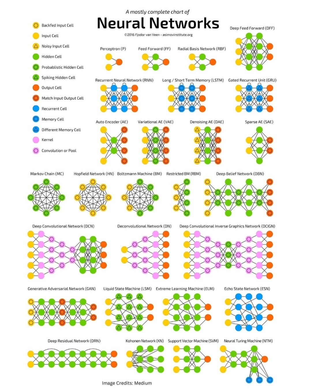
The field of neural networks is incredibly vast and continues to expand at an astonishing pace. What began with simple perceptrons has blossomed into a diverse ecosystem of architectures, each tailored to specific types of data and computational challenges. This “Neural Networks Zoo” chart serves as an excellent visual guide to this diversity, showcasing a wide array of network types, from the foundational to the cutting-edge.

This article aims to unpack this zoo, providing a detailed exploration of the various neural network architectures depicted in the chart. We will categorize them based on their fundamental design principles and applications, explaining their core mechanics, typical use cases, and how they differ from one another. By the end, you should have a clearer understanding of the rich tapestry that is the world of artificial neural networks.

The Fundamental Building Blocks: Cells and Operations

Before diving into specific network architectures, it’s crucial to understand the basic components that make up these complex systems. The chart uses a helpful legend to differentiate various “cells” and operations:

• Input Cell (Yellow Circle): Represents the entry point for data into the network. Each input cell typically corresponds to a feature in the input data (e.g., a pixel value in an image, a word in a sentence).
• Noisy Input Cell (Orange Circle): An input cell where noise is intentionally added to the input data. This can be used in techniques like denoising autoencoders to make the network more robust.
• Backfed Input Cell (Green Circle with inner yellow circle): An input cell that receives feedback from later layers or even the output layer. This implies a recurrent connection.
• Hidden Cell (Green Circle): The workhorse of a neural network. These cells process information between the input and output layers, learning complex patterns and representations. A network can have multiple hidden layers.
• Probabilistic Hidden Cell (Dark Green Circle): A hidden cell whose activation is determined probabilistically rather than deterministically. Often seen in generative models like Boltzmann Machines.
• Spiking Hidden Cell (Light Green Circle with spike): Inspired by biological neurons, these cells activate only when their internal potential reaches a certain threshold, producing discrete “spikes” of output. Found in Spiking Neural Networks (SNNs).
• Output Cell (Red Triangle): The final layer of the network, producing the network’s prediction or classification. The number of output cells depends on the task (e.g., one for binary classification, multiple for multi-class classification).
• Match Input Output Cell (Blue Circle): An output cell that aims to reconstruct or match the original input. This is characteristic of autoencoders, where the network learns to compress and decompress data.
• Recurrent Cell (Dark Blue Circle): A cell that has a connection back to itself or to a previous layer, allowing information to persist and influence future predictions. Essential for processing sequential data.
• Memory Cell (Light Blue Circle): A specialized recurrent cell designed to store and manage information over long sequences, addressing the vanishing/exploding gradient problem in traditional RNNs. Key to LSTMs and GRUs.
• Different Memory Cell (Purple Circle): Indicates another type of memory cell, likely with a slightly different internal gating mechanism than the standard memory cell.
• Kernel (Pink Square): Represents a small matrix of weights that slides over input data (e.g., an image) to perform convolution, extracting features.
• Convolution or Pool (Purple Square): Denotes a convolutional layer or a pooling layer, both fundamental operations in Convolutional Neural Networks (CNNs) for feature extraction and dimensionality reduction.

Understanding these symbols is key to interpreting the architectural diagrams of the networks in the zoo.

I. Foundational Architectures: The Building Blocks of Deep Learning

These networks represent some of the earliest and most fundamental neural network designs, laying the groundwork for more complex architectures.

1. Perceptron (P)

• Architecture: The simplest form of a neural network, consisting of one or more input cells and a single output cell. There are no hidden layers. Each input is multiplied by a weight, summed, and then passed through an activation function (typically a step function) to produce a binary output (0 or 1).
• Functionality: A perceptron is a linear classifier. It can learn to distinguish between two linearly separable classes.
• Limitations: Cannot solve non-linearly separable problems (e.g., XOR problem).
• Significance: While limited, the perceptron was a crucial step in the development of neural networks, demonstrating the ability of a simple computational unit to learn from data.

2. Feed Forward (FF) / Deep Feed Forward (DFF)

• Architecture: The most basic type of multi-layer neural network. Information flows in only one direction, from the input layer, through one or more hidden layers, to the output layer. There are no loops or cycles.
  • Feed Forward (FF): Typically refers to networks with one or a few hidden layers.
  • Deep Feed Forward (DFF): Implies networks with many hidden layers, leading to “deep” learning.
• Functionality: Universal function approximators. Given enough hidden units and layers, and appropriate activation functions, DFF networks can approximate any continuous function. They are widely used for classification, regression, and pattern recognition.
• Learning: Trained using backpropagation, an algorithm that calculates the gradient of the loss function with respect to the network’s weights, allowing for efficient weight updates.
• Applications: Image classification (for simpler tasks), natural language processing (for simpler tasks), tabular data analysis, and many other supervised learning problems.

3. Radial Basis Network (RBF)

• Architecture: Consists of an input layer, a hidden layer of radial basis functions, and an output layer. Unlike traditional feed-forward networks that use sigmoidal or ReLU activations in hidden layers, RBF networks use radial basis functions (e.g., Gaussian functions) in their hidden units. Each RBF unit has a center and a radius, and its activation decreases as the input moves away from its center.
• Functionality: Primarily used for function approximation, interpolation, and classification. They are particularly good at modeling non-linear relationships.
• Learning: Often trained in two phases: first, the centers and radii of the RBF units are determined (e.g., using clustering algorithms like K-means), and then the weights connecting the RBF layer to the output layer are learned.
• Applications: Time series prediction, control systems, medical diagnosis, and pattern recognition.

II. Recurrent Neural Networks (RNNs): Processing Sequences

Traditional feed-forward networks treat each input independently. However, many types of data, such as text, speech, and video, have a sequential nature where the order of information matters. Recurrent Neural Networks are designed to handle such sequential data by maintaining an internal “memory” of past inputs.

1. Recurrent Neural Network (RNN)

• Architecture: Characterized by recurrent connections, meaning that the output from a hidden layer at one time step is fed back as an input to the same hidden layer at the next time step. This allows information to persist across time.
• Functionality: Excellent for tasks involving sequences. They can map input sequences to output sequences, or a sequence to a single output (e.g., sentiment analysis of a sentence).
• Limitations:
  • Vanishing/Exploding Gradient Problem: During backpropagation through time (BPTT), gradients can become extremely small (vanishing) or extremely large (exploding) over long sequences, making it difficult for the network to learn long-range dependencies.
  • Short-Term Memory: Due to the vanishing gradient problem, basic RNNs struggle to remember information from inputs far back in the sequence.
• Applications: Speech recognition, machine translation, natural language generation, and time series prediction.

2. Long Short-Term Memory (LSTM)

• Architecture: A specialized type of RNN designed to overcome the vanishing gradient problem and better capture long-range dependencies. LSTMs introduce “memory cells” (the light blue circles in the diagram) and sophisticated “gates” (input gate, forget gate, output gate) that regulate the flow of information into and out of the memory cell.
  • Forget Gate: Decides what information to discard from the cell state.
  • Input Gate: Decides what new information to store in the cell state.
  • Output Gate: Decides what part of the cell state to output.
• Functionality: Highly effective at learning from and generating long sequences. The gates allow LSTMs to selectively remember or forget information, enabling them to maintain relevant context over extended periods.
• Significance: Revolutionized sequence modeling and became the go-to architecture for many NLP tasks before the advent of Transformers.
• Applications: Machine translation, speech recognition, sentiment analysis, text summarization, and video captioning.

3. Gated Recurrent Unit (GRU)

• Architecture: A simplified version of the LSTM, also designed to address the vanishing gradient problem. GRUs have fewer gates than LSTMs (typically a reset gate and an update gate), making them computationally less expensive while still achieving comparable performance in many tasks.
  • Update Gate: Controls how much of the previous hidden state should be carried over to the current hidden state.
  • Reset Gate: Determines how much of the previous hidden state to forget.
• Functionality: Similar to LSTMs in their ability to learn long-range dependencies in sequential data, but with a more streamlined structure.
• Significance: Offers a good balance between performance and computational efficiency, often preferred when computational resources are limited or for faster experimentation.
• Applications: Similar to LSTMs, widely used in NLP, speech processing, and time series analysis.

4. Liquid State Machine (LSM)

• Architecture: A type of Recurrent Neural Network that models a “liquid” of interconnected neurons. The “liquid” (a large, randomly connected recurrent neural network) receives input and generates a high-dimensional, transient response. A simpler, linear readout layer then learns to classify or regress based on this complex, dynamic “state” of the liquid. The internal connections of the liquid are typically fixed and untrained.
• Functionality: Designed for processing continuous, time-varying signals. They leverage the rich, dynamic responses of their recurrent “reservoir” to perform complex computations on temporal data.
• Key Idea: The “liquid” transforms the input into a high-dimensional, separable representation, which a simple linear classifier can then handle.
• Applications: Speech recognition, brain-computer interfaces, and other real-time signal processing tasks.

5. Echo State Network (ESN)

• Architecture: Similar in concept to Liquid State Machines. ESNs also use a “reservoir” of randomly connected recurrent neurons, but with sparse connections. The weights within the reservoir are fixed and randomly initialized, and only the weights connecting the reservoir to the output layer are trained.
• Functionality: Efficiently learn from and generate complex temporal patterns. Their fixed internal weights simplify training significantly compared to traditional RNNs.
• Key Idea: The “echo state property” ensures that the internal state of the reservoir is determined by the history of inputs, allowing for memory.
• Applications: Time series prediction, robot control, and signal processing.

III. Autoencoders (AEs): Learning Efficient Representations

Autoencoders are a type of neural network designed for unsupervised learning, specifically for learning efficient data encodings (representations). They aim to reconstruct their input, forcing the network to learn a compressed, meaningful representation in the process.

1. Auto Encoder (AE)

• Architecture: Consists of an encoder and a decoder.
  • Encoder: Maps the input data to a lower-dimensional latent space (the “bottleneck” or “code” layer, often the hidden layer in the middle).
  • Decoder: Maps the latent space representation back to the original input space.
• Functionality: The network is trained to minimize the reconstruction error between the input and its output. By forcing the data through a bottleneck, the autoencoder learns a compressed, feature-rich representation of the input.
• Applications: Dimensionality reduction, feature learning, anomaly detection (anomalies will have high reconstruction error), and data denoising.

2. Variational AE (VAE)

• Architecture: A generative model that builds upon the autoencoder concept by introducing a probabilistic approach to the latent space. Instead of learning a fixed encoding for each input, the encoder learns the parameters (mean and variance) of a probability distribution (typically Gaussian) in the latent space. The decoder then samples from this distribution to reconstruct the input.
• Functionality: VAEs are not only good at learning representations but also at generating new, similar data. By sampling from the learned latent distribution, they can produce novel outputs that resemble the training data.
• Key Idea: The latent space is regularized to ensure it is continuous and allows for smooth interpolation, making generation possible.
• Applications: Image generation, text generation, anomaly detection, and data imputation.

3. Denoising AE (DAE)

• Architecture: A variant of the autoencoder where the input is intentionally corrupted with noise (e.g., by randomly setting some pixel values to zero), and the network is trained to reconstruct the original, uncorrupted input.
• Functionality: Forces the network to learn more robust features that are less sensitive to noise. By learning to remove noise, the DAE effectively learns a more robust and meaningful representation of the underlying data.
• Applications: Feature learning, data denoising, and as a pre-training step for deep feed-forward networks.

4. Sparse AE (SAE)

• Architecture: An autoencoder where a sparsity constraint is imposed on the hidden layer activations. This means that only a small number of hidden units are allowed to be active (non-zero) for any given input.
• Functionality: Encourages the network to learn a more distributed representation where each hidden unit specializes in detecting a specific feature. This can lead to more interpretable features and better generalization.
• Applications: Feature learning, dimensionality reduction, and as a component in deep learning architectures.

IV. Probabilistic and Generative Models: Understanding and Creating Data

This category includes networks that explicitly model the probability distribution of the data, allowing them to understand underlying patterns and, in many cases, generate new data samples.

1. Markov Chain (MC)

• Architecture: While not strictly a neural network, Markov Chains are fundamental to understanding sequential data and probabilistic modeling, which underpin some neural network concepts. A Markov Chain is a stochastic model describing a sequence of possible events in which the probability of each event depends only on the state attained in the previous event.
• Functionality: Models systems that transition between states. The “memoryless” property (Markov property) is key.
• Relevance to NNs: Concepts like hidden Markov models (HMMs) were precursors to RNNs for sequence modeling. Probabilistic approaches are integrated into networks like Boltzmann Machines.
• Applications: Modeling natural language, weather prediction, financial modeling, and many other sequential processes.

2. Hopfield Network (HN)

• Architecture: A type of recurrent artificial neural network that serves as a content-addressable memory system. It consists of a single layer of interconnected neurons, where each neuron is connected to every other neuron. The connections are symmetric.
• Functionality: When an input pattern is presented, the network iteratively updates the states of its neurons until it converges to a stable state, which represents a stored memory. It can recall complete patterns from incomplete or noisy inputs.
• Key Idea: Energy function minimization. The network’s dynamics always lead to a local minimum of an energy function, corresponding to a stored memory.
• Applications: Associative memory, pattern completion, and optimization problems.

3. Boltzmann Machine (BM)

• Architecture: A type of recurrent neural network that is a stochastic (probabilistic) generative model. It consists of visible units (representing the input data) and hidden units (learning abstract features). All units are connected to all other units, and connections are symmetric.
• Functionality: Learns to model complex probability distributions over its inputs. It can be used for generative tasks (sampling new data) and for learning features. Training involves a process called “simulated annealing” or “contrastive divergence.”
• Limitations: Training full Boltzmann Machines is computationally very expensive due to the need to sample from the network’s equilibrium distribution.
• Applications: Feature learning, dimensionality reduction, and collaborative filtering.

4. Restricted Boltzmann Machine (RBM)

• Architecture: A simplified version of the Boltzmann Machine. The key restriction is that there are no connections between visible units and no connections between hidden units. Connections only exist between visible and hidden units.
• Functionality: Much easier to train than full Boltzmann Machines, typically using contrastive divergence. RBMs are powerful feature learners and can be stacked to form deeper networks.
• Significance: RBMs were a crucial component in the early success of deep learning, particularly in Deep Belief Networks, as they provided an effective way to pre-train layers in an unsupervised manner.
• Applications: Dimensionality reduction, collaborative filtering, feature learning, and as building blocks for Deep Belief Networks.

5. Deep Belief Network (DBN)

• Architecture: A generative deep neural network composed of multiple layers of Restricted Boltzmann Machines (RBMs) stacked on top of each other. The first RBM learns features from the raw input, the second RBM learns features from the features learned by the first RBM, and so on.
• Functionality: DBNs are trained greedily, layer by layer, in an unsupervised manner (each RBM learns to model its input). After pre-training, the entire network can be fine-tuned with supervised learning for tasks like classification.
• Significance: DBNs were among the first truly “deep” architectures that could be effectively trained, demonstrating the power of unsupervised pre-training for initializing deep networks.
• Applications: Image recognition, speech recognition, and information retrieval.

6. Generative Adversarial Network (GAN)

• Architecture: Consists of two competing neural networks:
  • Generator (G): Takes random noise as input and tries to generate realistic data samples (e.g., images).
  • Discriminator (D): Takes either real data samples or samples generated by the generator as input and tries to distinguish between them.
• Functionality: The two networks are trained in a zero-sum game. The generator tries to fool the discriminator into thinking its generated data is real, while the discriminator tries to get better at identifying fake data. This adversarial process leads to the generator producing increasingly realistic outputs.
• Significance: One of the most significant breakthroughs in generative AI, capable of producing incredibly realistic images, audio, and other data.
• Applications: Image generation (e.g., generating faces of non-existent people), image-to-image translation (e.g., converting sketches to photos), data augmentation, and super-resolution.

V. Convolutional Neural Networks (CNNs): Mastering Spatial Data

Convolutional Neural Networks are specifically designed to process data that has a known grid-like topology, such as images (2D grid of pixels) or time-series data (1D grid). They leverage the concept of shared weights and local receptive fields to efficiently learn hierarchical patterns.

1. Deep Convolutional Network (DCN)

• Architecture: Typically consists of multiple layers of:
  • Convolutional Layers (Pink Square): Apply learnable filters (kernels) that slide across the input, performing dot products to create feature maps. These filters detect local patterns like edges, textures, or specific shapes.
  • Pooling Layers (Purple Square): Reduce the spatial dimensions of the feature maps, helping to make the network robust to small shifts or distortions in the input. Common pooling operations include max pooling and average pooling.
  • Fully Connected Layers: After several convolutional and pooling layers, the learned features are flattened and fed into one or more standard feed-forward layers for classification or regression.
• Functionality: Highly effective at learning hierarchical representations from spatial data. Lower layers learn simple features, while higher layers combine these to learn more complex, abstract features.
• Significance: The backbone of modern computer vision, responsible for breakthroughs in image classification, object detection, and segmentation.
• Applications: Image classification, object detection, facial recognition, medical image analysis, and video analysis.

2. Deconvolutional Network (DN)

• Architecture: Can refer to a few related concepts:
  • Transposed Convolutional Network: Often used in the decoder part of autoencoders or in generative models. It performs the inverse operation of convolution, mapping a lower-dimensional representation to a higher-dimensional one, effectively “upsampling” or “deconvolving” feature maps.
  • Deconvolutional Neural Network (Zeiler & Fergus, 2014): A technique used to visualize and understand the features learned by a pre-trained CNN. It projects features from higher layers back to the input pixel space, revealing what patterns activate specific neurons.
• Functionality: Primarily used for generating images or reconstructing inputs from latent representations. When used for visualization, they help interpret CNNs.
• Applications: Image generation, semantic segmentation (where output needs to be pixel-level), and understanding CNN activations.

3. Deep Convolutional Inverse Graphics Network (DCIGN)

• Architecture: A type of generative model that combines elements of CNNs and inverse graphics. It aims to learn a disentangled representation of the underlying factors that generate an image (e.g., object identity, pose, lighting, texture).
• Functionality: Instead of just generating images, DCIGNs try to “understand” the generative process. They can take an image and infer its underlying graphical parameters, and then use these parameters to generate new images with controlled variations.
• Key Idea: It learns an inverse mapping from images to their underlying generative factors.
• Applications: Image manipulation, understanding image composition, and generating images with specific attributes.

VI. Other Notable Network Architectures and Concepts

The “zoo” also includes several other important architectures and machine learning concepts that are either specialized, foundational, or represent cutting-edge research directions.

1. Deep Residual Network (DRN)

• Architecture: Introduced the concept of “residual connections” or “skip connections.” Instead of learning a direct mapping from one layer to the next, residual blocks learn a “residual function” with respect to the input of the block. The input is added directly to the output of the block, bypassing one or more layers.
• Functionality: Solves the vanishing gradient problem and enables the training of extremely deep neural networks (hundreds or even thousands of layers). By allowing gradients to flow directly through the skip connections, information can propagate more easily throughout the network.
• Significance: A major breakthrough that allowed for the creation of much deeper and more powerful CNNs, leading to significant performance improvements in image recognition tasks.
• Applications: Image classification, object detection, and other computer vision tasks where very deep networks are beneficial.

2. Kohonen Network (KN) / Self-Organizing Map (SOM)

• Architecture: An unsupervised neural network that produces a low-dimensional (typically 2D) discretized representation of the input space, called a “map.” It consists of an input layer and an output layer (the “map” or “grid” of neurons). Each neuron on the map is connected to all input neurons.
• Functionality: Learns to map high-dimensional input data onto a lower-dimensional grid while preserving the topological properties of the input space. Neurons that are close to each other on the map will respond to similar input patterns.
• Learning: Uses a competitive learning process where the “winning” neuron (the one whose weights are closest to the input) and its neighbors are updated to move closer to the input.
• Applications: Data visualization, dimensionality reduction, clustering, and pattern recognition.

3. Support Vector Machine (SVM)

• Architecture: While not strictly a neural network in the traditional sense (it doesn’t have layers of interconnected “neurons” in the same way), SVMs are powerful supervised learning models often discussed alongside neural networks for classification and regression tasks. They are kernel-based methods.
• Functionality: SVMs aim to find the optimal hyperplane that best separates data points of different classes in a high-dimensional space. For non-linearly separable data, they use kernel functions to implicitly map the data into a higher-dimensional space where a linear separation is possible.
• Relevance to NNs: Often compared to NNs in terms of performance for certain tasks, and sometimes used in hybrid models.
• Applications: Classification (e.g., text categorization, image classification), regression, and outlier detection.

4. Neural Turing Machine (NTM)

• Architecture: A novel neural network architecture that combines a neural network controller (e.g., an LSTM or feed-forward network) with an external memory bank. The controller learns to read from and write to this memory, allowing it to perform complex algorithmic tasks.
• Functionality: Designed to mimic the computational capabilities of a Turing machine, allowing it to learn simple algorithms like copying, sorting, and associative recall. It aims to bridge the gap between neural networks and traditional computers.
• Key Idea: The external memory provides a form of long-term storage that is explicitly addressable by the network, overcoming the limited memory of standard RNNs.
• Applications: Learning algorithms, sequence processing where explicit memory manipulation is required, and potentially as a step towards more general AI.

5. Extreme Learning Machine (ELM)

• Architecture: A type of single-hidden layer feed-forward neural network where the weights connecting the input layer to the hidden layer are randomly assigned and never updated. The biases of the hidden neurons are also randomly assigned. Only the weights connecting the hidden layer to the output layer are learned.
• Functionality: Offers extremely fast training speeds because only the output weights need to be optimized. Despite random hidden layer weights, ELMs can still achieve good generalization performance due to the universal approximation theorem.
• Significance: Provides a computationally efficient alternative to traditional backpropagation-trained networks, especially for large datasets.
• Applications: Classification, regression, and pattern recognition, particularly in scenarios requiring fast training.

Conclusion: The Ever-Expanding Neural Networks Zoo

The “Neural Networks Zoo” chart provides a fascinating glimpse into the incredible diversity and ingenuity within the field of artificial intelligence. From the humble Perceptron to the sophisticated Generative Adversarial Networks and Neural Turing Machines, each architecture represents a solution to specific computational challenges and a step forward in our quest to build intelligent systems.

We’ve explored networks designed for:

• General-purpose pattern recognition and classification: Feed Forward Networks, RBF Networks.
• Processing sequential data and learning long-term dependencies: RNNs, LSTMs, GRUs, LSMs, ESNs.
• Learning efficient data representations and generating new data: Autoencoders (AE, VAE, DAE, SAE), Boltzmann Machines, RBMs, DBNs, GANs.
• Handling spatial data like images: DCNs, Deconvolutional Networks, DCIGNs, DRNs.
• Specialized tasks and algorithmic learning: Kohonen Networks, SVMs, NTMs, ELMs.

The rapid evolution of neural network architectures continues to push the boundaries of what AI can achieve. New models are constantly being developed, often combining elements from different architectures or introducing entirely new paradigms. Understanding the fundamental principles behind these “animals” in the neural network zoo is crucial for anyone looking to work with, understand, or contribute to the exciting world of artificial intelligence. As we move forward, the zoo will undoubtedly continue to grow, promising even more powerful and versatile intelligent systems.